没有合适的资源?快使用搜索试试~ 我知道了~
首页算法设计精要:Kleinberg与Tardos解析
算法设计精要:Kleinberg与Tardos解析
需积分: 8 5 下载量 82 浏览量
更新于2024-07-28
收藏 42.78MB PDF 举报
"算法设计 Kleinberg-Tardos"
《算法设计》是计算机科学领域的一本经典教材,由Cornell大学的Erik D. Demaine和János Pach两位教授撰写,书中深入探讨了算法设计技术和策略。这本书的目标是通过丰富的实例来阐述各种算法设计方法,帮助读者理解和应用这些技术解决实际问题。
全书围绕着算法设计的核心概念展开,包括分治法、动态规划、贪心算法、回溯法、近似算法和随机化算法等。每个主题都精心挑选了多个典型范例进行详尽分析,旨在让读者能够掌握每种技术的本质,并能灵活运用到实际的编程和问题解决中。
例如,分治法是一种将复杂问题分解成较小规模的相似子问题来求解的策略。在书中,作者会通过诸如快速排序、归并排序等经典算法,解释如何应用分治法来提高效率。动态规划则常用于优化有重叠子问题和最优子结构的问题,如背包问题和最长公共子序列问题。书中通过具体实例,演示如何构建状态转移方程和记忆化搜索。
贪心算法是每次选择当前看起来最优的决策,而不考虑未来可能的影响。书中可能会讨论霍夫曼编码、Prim最小生成树算法等,展示贪心策略如何在某些情况下达到全局最优。回溯法则是在面临多种选择时,尝试所有可能的路径,直到找到解决方案或确定无法找到解为止,如八皇后问题的解法。
近似算法是针对NP难问题的一种处理方式,因为这些问题在多项式时间内无法找到精确解。书中会讲解如何设计有效的近似算法,如最小割问题的网络流算法。最后,随机化算法利用概率理论来解决问题,如快速傅里叶变换(FFT)和舍伍德算法,它们在处理大规模数据时表现出色。
本书还包含了清晰的技术插图,以帮助读者直观理解复杂的算法过程。此外,严谨的排版和索引设计使得查阅和学习变得更加方便。无论你是初学者还是有经验的程序员,都能从中受益,提升自己的算法设计能力。
《算法设计 Kleinberg-Tardos》是一本全面介绍算法设计思想和技巧的教科书,对于想要在算法领域深化学习的人来说,它是一份不可多得的资源。通过阅读和实践书中的例子,读者可以系统地掌握算法设计的精髓,提高问题解决的能力。
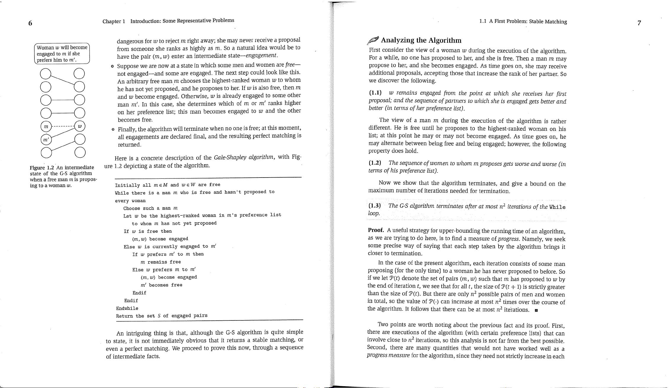
6
Chapter 1 Introduction: Some Representative Problems
1.1 A First Problem: Stable Matching
7
I~
oman w will become~
ngaged to m if she
|
refers him to rat
J
©
©
©
Figure 1.2 An intermediate
state of the G-S algorithm
when a free man ra is propos-
ing to a woman w.
dangerous for w to reject m right away; she may never receive a proposal
from someone she ranks as highly as m. So a natural idea would be to
have the pair
(m, w)
enter an intermediate
state--engagement.
Suppose we are now at a state in which some men and women are/Tee--
not engaged--and some are engaged. The next step could look like this.
An arbitrary flee man m chooses the highest-ranked woman w to whom
he has not yet proposed, and he proposes to her. If w is also free, then m
and w become engaged. Otherwise, w is already engaged to some other
man m’. In this case, she determines which of m or m’ ranks higher
on her preference list; this man becomes engaged to w and the other
becomes flee,
Finally, the algorithm wil! terminate when no one is free; at this moment,
all engagements are declared final, and the resulting perfect matchdng is
returned.
Here is a concrete description of the
Gale-Shapley algorithm, with
Fig-
ure 1.2 depicting a state of the algorithm.
Initially all m E M and w E W are free
While there is a man m who is free and hasn’t proposed to
every woman
Choose such a man m
Let w be the highest-ranked woman in m’s preference list
to whom m has not yet proposed
If ~ is free then
(m, ~) become engaged
Else ~ is currently engaged to m’
If ~ prefers m’ to m then
m remains free
Else w prefers m to m’
(m,~) become engaged
nl
I
becomes free
Endif
Endif
Endwhile
Return the set S of engaged pairs
An intriguing thing is that, although the G-S algorithm is quite simple
to state, it is not immediately obvious that it returns a stable matching, or
even a perfect matching. We proceed to prove this now, through a sequence
of intermediate facts.
~ Analyzing the Algorithm
First consider the view of a woman w during the execution of the algorithm.
For a while, no one has proposed to her, and she is free. Then a man m may
propose to her, and she becomes engaged. As time goes on, she may receive
additional proposals, accepting those that increase the rank of her partner. So
we discover the following.
(1.1)
w remains engaged /Tom the point at which she receives her first
proposal; and the sequence of partners to which she is engaged gets better and
better (in terms of her preference list).
The view of a man m during the execution of the algorithm is rather
different. He is free until he proposes to the highest-ranked woman on his
list; at this point he may or may not become engaged. As time goes on, he
may alternate between being free and being engaged; however, the following
property does hold.
(1.2)
The sequence of women to whom m proposes gets worse and worse (in
terms of his preference list).
Now we show that the algorithm terminates, and give a bound on the
maximum number of iterations needed for termination.
(1,3)
The G-S algorithm terminates after at most n
2
iterations of the
While
loop.
Proof. A useful strategy for upper-bounding the running time of an algorithm,
as we are trying to do here, is to find a measure of
progress.
Namely, we seek
some precise way of saying that each step taken by the algorithm brings it
closer to termination.
In the case of the present algorithm, each iteration consists of some man
proposing (for the only time) to a woman he has never proposed to before. So
if we let ~P(t) denote the set of pairs
(m, w)
such that m has proposed to w by
the end of iteration
t,
we see that for all
t, the
size of ~P(t + 1) is strictly greater
than the size of ~P(t). But there are only n
2
possible pairs of men and women
in total, so the value of ~P(.) can increase at most n
2
times over the course of
the algorithm. It follows that there can be at most n
2
iterations. []
Two points are worth noting about the previous fact and its proof. First,
there are executions of the algorithm (with certain preference lists) that can
involve close to n
2
iterations, so this analysis is not far from the best possible.
Second, there are many quantities that would not have worked well as a
progress measure
for the algorithm, since they need not strictly increase in each
8
Chapter 1 Introduction: Some Representative Problems
1.1 A First Problem: Stable Matching
9
iteration. For example, the number of free individuals could remain constant
from one iteration to the next, as could the number of engaged pairs. Thus,
these quantities could not be used directly in giving an upper bound on the
maximum possible number of.iterations, in the style of the previous paragraph.
Let us now establish that the set S returned at the termination of the
algorithm is in fact a perfect matching. Why is this not immediately obvious?
Essentially, we have to show that no man can
"fall
off" the end of his preference
list; the only way for the ~’h±].e loop to exit is for there to be no flee man. In
this case, the set of engaged couples would indeed be a perfect matching.
So the main thing we need to show is the following.
(1.4)
If m is free at some point in the execution of the algorithm, then there
is a woman to whom he has not yet proposed.
Proof. Suppose there comes a point when m is flee but has already proposed
to every woman. Then by (1.1), each of the n women is engaged at this point
in time. Since the set of engaged pairs forms a matching, there must also be
n engaged men at this point in time. But there are only n men total, and m is
not engaged, so this is a contradiction.
,,
(1..~)
The set S returned at termination is a peryect matching.
Proof. The set of engaged pairs always forms a matching. Let us suppose that
the algorithm terminates with a flee man m. At termination, it must be the
case that m had already proposed to every woman, for otherwise the ~qhile
loop would not have exited. But this contradicts (1.4), which says that there
cannot be a flee man who has proposed to every woman.
,,
Finally, we prove the main property of the algorithm--namely, that it
results in a stable matching.
(1.6)
Consider an executionof the G-S algorithm that returns a set of pairs
S. The set S is a stable matching.
Proof. We have already seen, in (1.5), that S is a perfect matching. Thus, to
prove S is a stable matching, we will assume that there is an instability with
respect to S and obtain a contradiction. As defined earlier, such an instability
would involve two pairs,
(m, w)
and (m’, w’), in S with the properties that
o m prefers w’ to w, and
o w’ prefers m to mL
In the execution of the algorithm that produced S, m’s last proposal was, by
definition, to w. Now we ask: Did m propose to w’ at some earlier point in
this execution? If he didn’t, then w must occur higher on
m’s
preference.list
than w’,
contxadicting our assumption that m prefers w’ to w. If he did, then
he was rejected by w’ in favor of some other man
m",
whom w’ prefers to m.
m’
is the final partner of
w’,
so either m" = m’ or, by (1.!), w’ prefers her final
partner m
~
to m"; either way this contradicts our assumption that w’ prefers
m to m
I.
It follows that S is a stable matching. []
Extensions
We began by defining the notion of a stable matching; we have just proven
that the G-S algorithm actually constructs one. We now consider some further
questions about the behavior of the G-S algorithm and its relation to the
properties of different stable matchings.
To begin wit_h, recall that we saw an example earlier in which there could
be multiple stable matchings. To recap, the preference lists in this example
were as follows:
prefers w to w’.
~
prefers w’ to w.
prefers m
~
to m.
prefers m to m’.
Now, in any execution of the Gale-Shapley algorithm, m will become engaged
to
w, m’ will become engaged to w’ (perhaps in the other order), and things
will stop there. Thus, the
other
stable matching, consisting of the pairs
(m’, w)
and
(m, w’),
is not attainable from an execution of the G-S algorithm in which
the men propose. On the other hand, it would be reached if we ran a version of
the algorithm in which the women propose. And in larger examples, with more
than two people on each side, we can have an even larger collection of possible
stable matchings, many of them not achievable by any natural algorithm.
This example shows a certain "unfairness" in the G-S algorithm, favoring
men. If the men’s preferences mesh perfectly (they all list different women as
their first choice), then in all runs of the G-S algorithm all men end up matched
with their first choice, independent of the preferences of the women. If the
women’s preferences clash completely with the men’s preferences (as was the
case in this example), then the resulting stable matching is as bad as possible
for the women. So this simple set of preference lists compactly summarizes a
world in which
someone
is destined to end up unhappy: women are unhappy
if men propose, and men are unhappy if women propose.
Let’s now analyze the G-S algorithm in more detail and try to understand
how general this "unfairness" phenomenon is.
10
Chapter 1 Introduction: Some Representative Problems
To begin With, our example reinforces the point that the G-S algorithm
is actually underspecified: as long as there is a free man, we are allowed to
choose any flee man to make the next proposal. Different choices specify
different executions of the algprithm; this is why, to be careful, we stated (1.6)
as "Consider an execution of the G-S algorithm that returns a set of pairs
S,"
instead of "Consider the set S returned by the G-S algorithm."
Thus, we encounter another very natural question: Do all executions of
the G-S algorithm yield the same matching? This is a genre of question that
arises in many settings in computer science: we have an algorithm that runs
asynchronously,
with different independent components performing actions
that can be interleaved in complex ways, and we want to know how much
variability this asynchrony causes in the final outcome. To consider a very
different kind of example, the independent components may not be men and
women but electronic components activating parts of an airplane wing; the
effect of asynchrony in their behavior can be a big deal.
In the present context, we will see that the answer to our question is
surprisingly clean: all executions of the G-S algorithm yield the same matching.
We proceed to prove this now.
All Executions Yield the Same Matching
There are a number of possible
ways to prove a statement such as this, many of which would result in quite
complicated arguments. It turns out that the easiest and most informative ap-
proach for us will be to uniquely
characterize the
matching that is obtained and
then show that al! executions result in the matching with this characterization.
What is the characterization? We’ll show that each man ends up with the
"best possible partner" in a concrete sense. (Recall that this is true if all men
prefer different women.) First, we will say that a woman iv is a
valid partner
of a man m if there is a stable matching that contains the pair
(m, iv).
We will
say that iv is the
best valid partner
of m if iv is a valid parmer of m, and no
woman whom m ranks higher than iv is a valid partner of his. We will use
best(m)
to denote the best valid partner of m.
Now, let S* denote the set of pairs {(m,
best(m)) : m ~ M}.
We will prove
the folloWing fact.
(1.7)
Every execution of the C--S algorithm results in the set S*:
This statement is surprising at a number of levels. First of all, as defined,
there is no reason to believe that S* is a matching at all, let alone a stable
matching. After all, why couldn’t it happen that two men have the same best
valid partner? Second, the result shows that the G-S algorithm gives the best
possible outcome for every man simultaneously; there is no stable matching
in which any of the men could have hoped to do better. And finally, it answers
1.1 A First Problem: Stable Matching
our question above by showing that the order of proposals in the G-S algorithm
has absolutely no effect on the final outcome.
Despite all this, the proof is not so difficult.
Proof. Let us suppose, by way of contradiction, that some execution g of the
G-S algorithm results in a matching S in which some man is paired with a
woman who is not his best valid partner. Since men propose in decreasing
order of preference, this means that some man is rejected by a valid partner
during the execution g of the algorithm. So consider the first moment during
the execution g in which some man, say m, is rejected by a valid partner iv.
Again, since men propose in decreasing order of preference, and since this is
the first time such a rejection has occurred, it must be that iv is m’s best valid
partner
best(m).
The reiection of m by iv may have happened either because m proposed
and was turned down in favor of iv’s existing engagement, or because iv broke
her engagement to m in favor of a better proposal. But either way, at this
moment iv forms or continues an engagement with a man m’ whom she prefers
to m.
Since iv is a valid parmer of m, there exists a stable matching S’ containing
the pair (m, iv).
Now we ask: Who is m’ paired with in this matching? Suppose
it is a woman
iv’ ~= iv.
Since the rejection of m by iv was the first rejection of a man by a valid
partner in the execution ~, it must be that m’ had not been rejected by any valid
parmer at the point in ~ when he became engaged to iv. Since he proposed in
decreasing order of preference, and since iv’ is clearly a valid parmer of m’,
it
must be that m’ prefers iv to
iv’.
But we have already seen that iv prefers m’
to m, for in execution ~ she rejected m in favor of m’. Since (m’, iv)
S’,
it
follows that (m’, iv) is an instability in S’.
This contradicts our claim that S’ is stable and hence contradicts our initial
assumption. []
So for the men, the G-S algorithm is ideal. Unfortunately, the same cannot
be said for the women. For a woman w, we say that m is a valid partner if
there is a stable matching that contains the pair (m, w). We say that m is the
ivorst valid partner
of iv if m is a valid partner of
w,
and no man whom iv
ranks lower than m is a valid partner of hers.
(1.8)
In the stable matching S*, each woman is paired ivith her ivorst valid
partner.
Proof.
Suppose there were a pair (m, iv) in S* such that m is not the worst
valid partner of iv. Then there is a stable matching S’ in which iv is paired
11
12
Chapter
1 Introduction: Some Representative Problems
with a man m’ whom she likes less than m. In S’, m is paired with a woman
w’ ~ w; since w is the best valid partner of m, and w’ is a valid partner of
m,
we see that m prefers w to w’.
But from this it follows that (m, w) is an instability in S’, contradicting the
claim that S’ is stable and hence contradicting our initial assumption. []
Thus, we find that our simple example above, in which the men’s pref-
erences clashed with the women’s, hinted at a very general phenomenon: for
any input, the side that does the proposing in the G-S algorithm ends up with
the best possible stable matching (from their perspective), while the side that
does not do the proposing correspondingly ends up with the worst possible
stable matching.
1.2 Five Representative Problems
The Stable Matching Problem provides us with a rich example of the process of
algorithm design. For many problems, this process involves a few significant,
steps: formulating the problem with enough mathematical precision that we
can ask a concrete question and start thinking about algorithms to solve
it; designing an algorithm for the problem; and analyzing the algorithm by
proving it is correct and giving a bound on the running time so as to establish
the algorithm’s efficiency.
This high-level strategy is carried out in practice with the help of a few
fundamental design techniques, which are very useful in assessing the inherent
complexity of a problem and in formulating an algorithm to solve it. As in any
area, becoming familiar with these design techniques is a gradual process; but
with experience one can start recognizing problems as belonging to identifiable
genres and appreciating how subtle changes in the statement of a problem can
have an enormous effect on its computational difficulty.
To get this discussion started, then,, it helps to pick out a few representa-
tive milestones that we’ll be encountering in our study of algorithms: cleanly
formulated problems, all resembling one another at a general level, but differ-
ing greatly in their difficulty and in the kinds of approaches that one brings
to bear on them. The first three will be solvable efficiently by a sequence of
increasingly subtle algorithmic techniques; the fourth marks a major turning
point in our discussion, serving as an example of a problem believed to be un-
solvable by any efficient algorithm; and the fifth hints at a class of problems
believed to be harder stil!.
The problems are self-contained and are al! motivated by computing
applications. To talk about some of them, though, it will help to use the
termino!ogy of
graphs.
While graphs are a common topic in earlier computer
1.2 Five Representative Problems
science courses, we’ll be introducing them in a fair amount of depth in
Chapter 3; due to their enormous expressive power, we’ll also be using them
extensively throughout the book. For the discussion here, it’s enough to think
of a graph G as simply a way of encoding pairwise relationships among a set
of objects. Thus, G consists of a pair of sets
(V,
E)--a collection V of
nodes
and a collection E of
edges, each of which "joins" two of the nodes. We thus
represent an edge e ~ E as a two-element subset of V: e =
(u, u)
for some
u, u ~ V,
where we call u and u the
ends
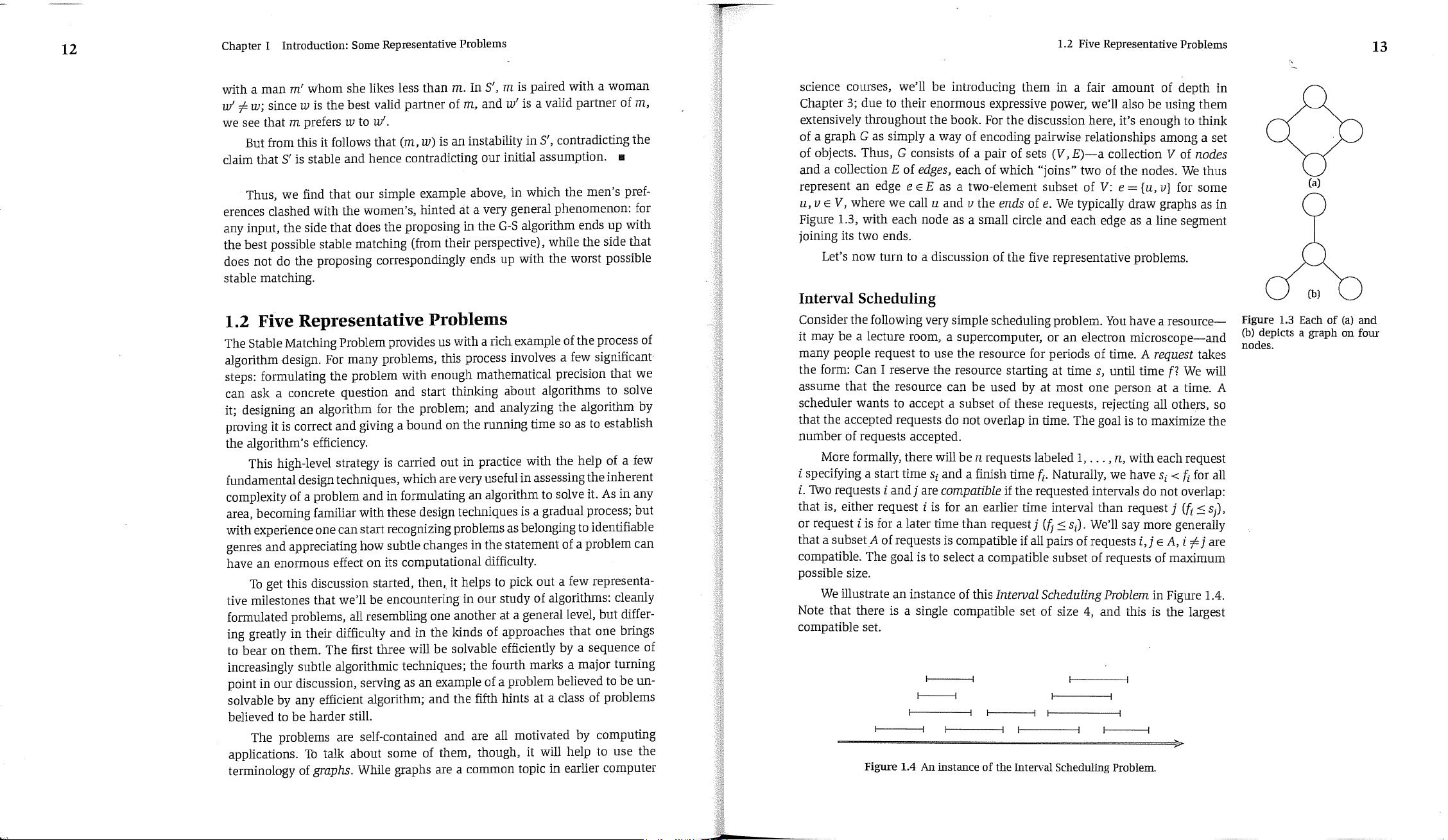
of e. We typica!ly draw graphs as in
Figure 1.3, with each node as a small circle and each edge as a line segment
joining its two ends.
Let’s now turn to a discussion of the five representative problems.
Interval Scheduling
Consider the following very simple scheduling problem. You have a resource--
it may be a lecture room, a supercompnter, or an electron microscope--and
many people request to use the resource for periods of time. A
request
takes
the form: Can I reserve the resource starting at time
s,
until time f? We will
assume that the resource can be used by at most one person at a time. A
scheduler wants to accept a subset of these requests, rejecting al! others, so
that the accepted requests do not overlap in time. The goal is to maximize the
number of requests accepted.
More formally, there will be n requests labeled 1 ..... n, with each request
i specifying a start time
si
and a finish time fi. Naturally, we have si < fi for all
i. Two requests i andj are
compatible
if the requested intervals do not overlap:
that is, either request i is for an earlier time interval than request
j (fi
<
or request i is for a later time than request j (1~ _< si). We’ll say more generally
that a subset A of requests is compatible if all pairs of requests
i,j ~ A, i ~=j are
compatible. The goal is to select a compatible subset of requests of maximum
possible size.
We illustrate an instance of this
Interual Scheduling Problem
in Figure 1.4.
Note that there is a single compatible set of size 4, and this is the largest
compatible set.
Figure 1.4 An instance of the Interval Scheduling Problem.
(a)
13
Figure 1.3 Each of (a) and
(b) depicts a graph on four
nodes.
14
Chapter ! Introduction: Some Representative Problems
We will see shortly that this problem can be solved by a very natural
algorithm that orders the set of requests according to a certain heuristic and
then "greedily" processes them in one pass, selecting as large a compatible
subset as it can. This will be .typical of a class of
greedy algorithms
that we
will consider for various problems--myopic rules that process the input one
piece at a time with no apparent look-ahead. When a greedy algorithm can be
shown to find an optimal solution for al! instances of a problem, it’s often fairly
surprising. We typically learn something about the structure of the underlying
problem from the fact that such a simple approach can be optimal.
Weighted Interval Scheduling
In the Interval Scheduling Problem, we sohght to maximize the
number
of
requests that could be accommodated simultaneously. Now, suppose more
generally that each request interval i has an associated
value,
or
weight,
vi > O; we could picture this as the amount of money we will make from
the
i
th
individual if we schedule his or her request. Our goal will be to find a
compatible subset of intervals of maximum total value.
The case in which vi = I for each i is simply the basic Interval Scheduling
Problem; but the appearance of arbitrary values changes the nature of the
maximization problem quite a bit. Consider, for example, that if v
1
exceeds
the sum of all other vi, then the optimal solution must include interval 1
regardless of the configuration of the fi~l set of intervals. So any algorithm
for this problem must be very sensitive to the values, and yet degenerate to a
method for solving (unweighted) interval scheduling when all the values are
equal to 1.
There appears to be no simple greedy rule that walks through the intervals
one at a time, making the correct decision in the presence of arbitrary values.
Instead, we employ a technique,
dynamic programming,
that builds up the
optimal value over all possible solutions in a compact, tabular way that leads
to a very efficient algorithm.
Bipal~te Matching
When we considered the Stable Matching Problem, we defined a
matching
to
be a set of ordered pairs of men and women with the property that each man
and each woman belong to at most one of the ordered pairs. We then defined
a perfect matching to be a matching in which every man and every woman
belong to some pair.
We can express these concepts more generally in terms of graphs, and in
order to do this it is useful to define the notion of a
bipartite graph.
We say that
a graph G ---- (V, E) is
bipa~te
if its node set V can be partitioned into sets X
1.2 Five Representative Problems
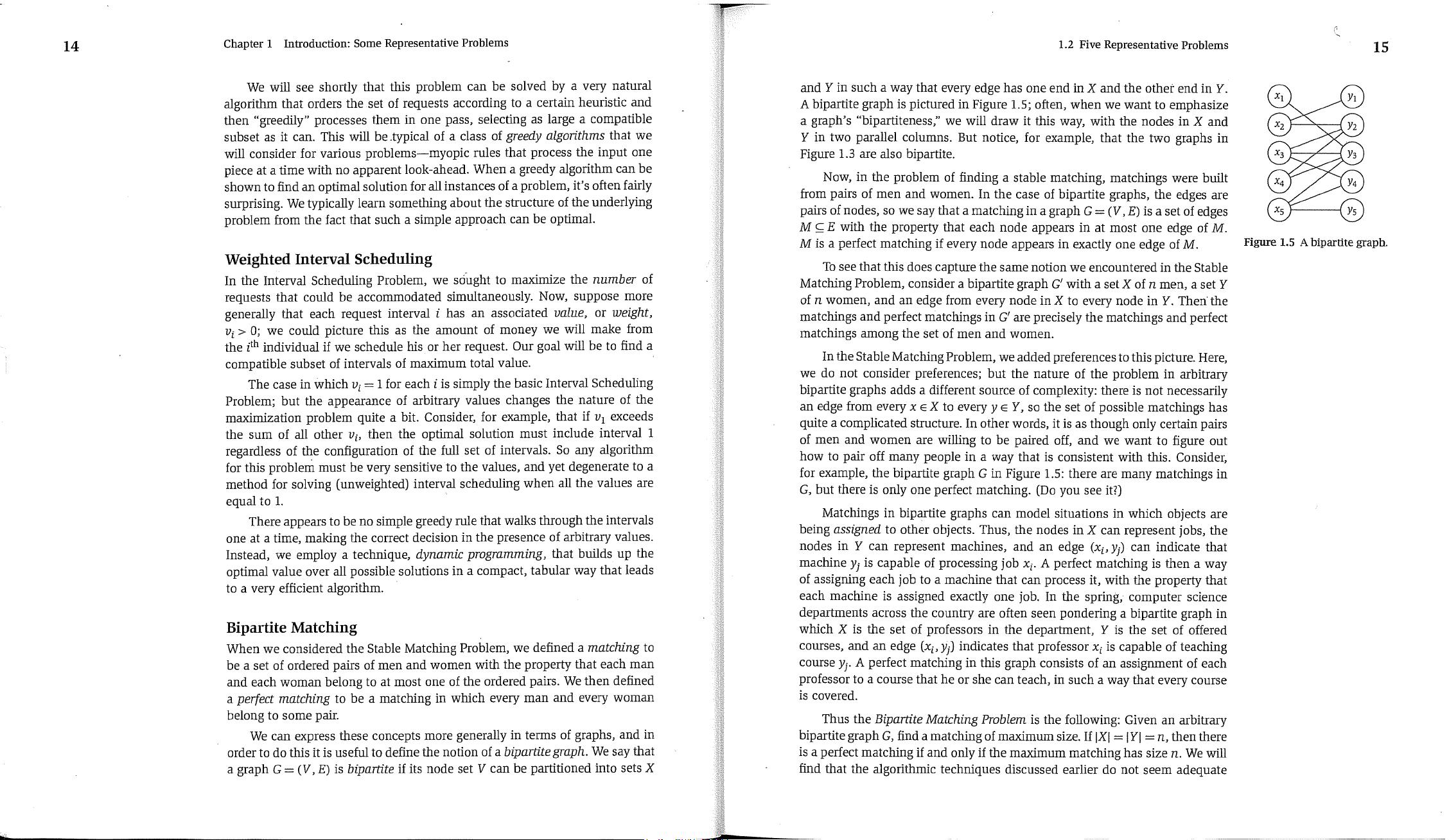
and Y in such a way that every edge has one end in X and the other end in Y.
A bipartite graph is pictured in Figure 1.5; often, when we want to emphasize
a graph’s "bipartiteness," we will draw it this way, with the nodes in X and
Y in two parallel columns. But notice, for example, that the two graphs in
Figure 1.3 are also bipartite.
Now, in the problem of finding a stable matching, matchings were built
from pairs of men and women. In the case of bipartite graphs, the edges are
pairs of nodes, so we say that a matching in a graph G = (V, E) is a set of edges
M _c E with the property that each node appears in at most one edge of M.
M is a perfect matching if every node appears in exactly one edge of M.
To see that this does capture the same notion we encountered in the Stable
Matching Problem, consider a bipartite graph G’ with a set X of n men, a set Y
of n women, and an edge from every node in X to every node in Y. Then the
matchings and perfect matchings in G’ are precisely the matchings and perfect
matchings among the set of men and women.
In the Stable Matching Problem, we added preferences to this picture. Here,
we do not consider preferences; but the nature of the problem in arbitrary
bipartite graphs adds a different source of complexity: there is not necessarily
an edge from every x ~ X to every y ~ Y, so the set of possible matchings has
quite a complicated structure. In other words, it is as though only certain pairs
of men and women are willing to be paired off, and we want to figure out
how to pair off many people in a way that is consistent with this. Consider,
for example, the bipartite graph G in Figure 1.5: there are many matchings in
G, but there is only one perfect matching. (Do you see it?)
Matchings in bipartite graphs can model situations in which objects are
being
assigned
to other objects. Thus, the nodes in X can represent jobs, the
nodes in Y can represent machines, and an edge (x~, y]) can indicate that
machine y] is capable of processing job xi. A perfect matching is then a way
of assigning each job to a machine that can process it, with the property that
each machine is assigned exactly one job. In the spring, computer science
departments across the country are often seen pondering a bipartite graph in
which X is the set of professors in the department, Y is the set of offered
courses, and an edge (xi, yj) indicates that professor x~ is capable of teaching
course y]. A perfect matching in this graph consists of an assignment of each
professor to a course that he or she can teach, in such a way that every course
is covered.
Thus the
Bipartite Matching Problem
is the following: Given an arbitrary
bipartite graph
G,
find a matching of maximum size. If IXI = I YI = n, then there
is a perfect matching if and only if the maximum matching has size n. We will
find that the algorithmic techniques discussed earlier do not seem adequate
15
Figure 1.5 A bipartite graph.
剩余431页未读,继续阅读
2018-03-21 上传
138 浏览量
2019-12-18 上传
点击了解资源详情
2021-03-17 上传
2021-06-03 上传
点击了解资源详情
点击了解资源详情
点击了解资源详情
fly_high_in_sky
- 粉丝: 0
- 资源: 5
上传资源 快速赚钱
 我的内容管理
展开
 我的资源
快来上传第一个资源
 我的收益 登录查看自己的收益
 我的积分
登录查看自己的积分
 我的C币
登录后查看C币余额
 我的收藏
我的收藏  我的下载
我的下载  下载帮助
下载帮助

最新资源
- Java毕业设计项目:校园二手交易网站开发指南
- Blaseball Plus插件开发与构建教程
- Deno Express:模仿Node.js Express的Deno Web服务器解决方案
- coc-snippets: 强化coc.nvim代码片段体验
- Java面向对象编程语言特性解析与学生信息管理系统开发
- 掌握Java实现硬盘链接技术:LinkDisks深度解析
- 基于Springboot和Vue的Java网盘系统开发
- jMonkeyEngine3 SDK:Netbeans集成的3D应用开发利器
- Python家庭作业指南与实践技巧
- Java企业级Web项目实践指南
- Eureka注册中心与Go客户端使用指南
- TsinghuaNet客户端:跨平台校园网联网解决方案
- 掌握lazycsv:C++中高效解析CSV文件的单头库
- FSDAF遥感影像时空融合python实现教程
- Envato Markets分析工具扩展:监控销售与评论
- Kotlin实现NumPy绑定:提升数组数据处理性能
安全验证
文档复制为VIP权益,开通VIP直接复制
 信息提交成功