numTest = length(imdsTest.Files); for i = 1:numTest testImage = readimage(imdsTest,i);
时间: 2024-05-29 19:14:05 浏览: 10
这段代码是用于读取测试集中的图像数据。首先,通过`length(imdsTest.Files)`获取测试集中图像文件的数量,存储在`numTest`变量中。然后,使用`for`循环遍历每一个测试图像,在循环体中使用`readimage`函数读取对应的图像数据,存储在`testImage`变量中。这样就能够逐一获取测试集中的所有图像数据,用于后续的模型测试和评估。
相关问题
这是对单个文件进行预测“import os import json import torch from PIL import Image from torchvision import transforms import matplotlib.pyplot as plt from model import convnext_tiny as create_model def main(): device = torch.device("cuda:0" if torch.cuda.is_available() else "cpu") print(f"using {device} device.") num_classes = 5 img_size = 224 data_transform = transforms.Compose( [transforms.Resize(int(img_size * 1.14)), transforms.CenterCrop(img_size), transforms.ToTensor(), transforms.Normalize([0.485, 0.456, 0.406], [0.229, 0.224, 0.225])]) # load image img_path = "../tulip.jpg" assert os.path.exists(img_path), "file: '{}' dose not exist.".format(img_path) img = Image.open(img_path) plt.imshow(img) # [N, C, H, W] img = data_transform(img) # expand batch dimension img = torch.unsqueeze(img, dim=0) # read class_indict json_path = './class_indices.json' assert os.path.exists(json_path), "file: '{}' dose not exist.".format(json_path) with open(json_path, "r") as f: class_indict = json.load(f) # create model model = create_model(num_classes=num_classes).to(device) # load model weights model_weight_path = "./weights/best_model.pth" model.load_state_dict(torch.load(model_weight_path, map_location=device)) model.eval() with torch.no_grad(): # predict class output = torch.squeeze(model(img.to(device))).cpu() predict = torch.softmax(output, dim=0) predict_cla = torch.argmax(predict).numpy() print_res = "class: {} prob: {:.3}".format(class_indict[str(predict_cla)], predict[predict_cla].numpy()) plt.title(print_res) for i in range(len(predict)): print("class: {:10} prob: {:.3}".format(class_indict[str(i)], predict[i].numpy())) plt.show() if name == 'main': main()”,改为对指定文件夹下的左右文件进行预测,并绘制混淆矩阵,
好的,为了实现您的需求,您需要进行以下几个步骤:
1. 加载模型和类别标签:
您需要在代码中加载您的模型和类别标签。您可以使用之前的代码中的方式来加载它们,只需要做一些小的改动即可。例如,您需要将模型和类别标签的路径作为参数传递给您的函数。
2. 加载测试集:
您需要加载您的测试集。您可以使用 `torchvision.datasets.ImageFolder` 来加载测试集。这个函数会将每个文件夹中的所有图像文件都加载到一个 tensor 中,并自动为每个文件夹分配一个标签。
3. 进行预测:
您需要对测试集中的每个图像进行预测,并将预测结果与真实标签进行比较。您可以使用之前的代码中的方式来预测每个图像,只需要做一些小的改动即可。例如,您需要将预测结果保存到一个列表中,并将真实标签保存到另一个列表中。
4. 绘制混淆矩阵:
最后,您需要使用预测结果和真实标签来绘制混淆矩阵。您可以使用 `sklearn.metrics.confusion_matrix` 来计算混淆矩阵,并使用 `matplotlib` 来绘制它。
下面是修改后的代码示例:
```
import os
import json
import torch
from PIL import Image
from torchvision import transforms
import matplotlib.pyplot as plt
from sklearn.metrics import confusion_matrix
import numpy as np
from model import convnext_tiny as create_model
def predict_folder(model_path, json_path, folder_path):
device = torch.device("cuda:0" if torch.cuda.is_available() else "cpu")
print(f"using {device} device.")
num_classes = 5
img_size = 224
data_transform = transforms.Compose([
transforms.Resize(int(img_size * 1.14)),
transforms.CenterCrop(img_size),
transforms.ToTensor(),
transforms.Normalize([0.485, 0.456, 0.406], [0.229, 0.224, 0.225])
])
# load class_indict json
with open(json_path, "r") as f:
class_indict = json.load(f)
# create model
model = create_model(num_classes=num_classes).to(device)
# load model weights
model.load_state_dict(torch.load(model_path, map_location=device))
model.eval()
y_true = []
y_pred = []
for root, dirs, files in os.walk(folder_path):
for file in files:
if file.endswith(".jpg") or file.endswith(".jpeg"):
img_path = os.path.join(root, file)
assert os.path.exists(img_path), "file: '{}' dose not exist.".format(img_path)
img = Image.open(img_path)
# [N, C, H, W]
img = data_transform(img)
# expand batch dimension
img = torch.unsqueeze(img, dim=0)
# predict class
with torch.no_grad():
output = torch.squeeze(model(img.to(device))).cpu()
predict = torch.softmax(output, dim=0)
predict_cla = torch.argmax(predict).numpy()
y_true.append(class_indict[os.path.basename(root)])
y_pred.append(predict_cla)
# plot confusion matrix
cm = confusion_matrix(y_true, y_pred)
fig, ax = plt.subplots(figsize=(5, 5))
ax.imshow(cm, cmap=plt.cm.Blues, aspect='equal')
ax.set_xlabel('Predicted label')
ax.set_ylabel('True label')
ax.set_xticks(np.arange(len(class_indict)))
ax.set_yticks(np.arange(len(class_indict)))
ax.set_xticklabels(class_indict.values(), rotation=90)
ax.set_yticklabels(class_indict.values())
ax.tick_params(axis=u'both', which=u'both',length=0)
for i in range(len(class_indict)):
for j in range(len(class_indict)):
text = ax.text(j, i, cm[i, j], ha="center", va="center", color="white" if cm[i, j] > cm.max() / 2. else "black")
fig.tight_layout()
plt.show()
if __name__ == '__main__':
# set the paths for the model, class_indict json, and test data folder
model_path = './weights/best_model.pth'
json_path = './class_indices.json'
folder_path = './test_data'
predict_folder(model_path, json_path, folder_path)
```
请注意,这个函数的参数需要您自己根据您的实际情况进行设置,以匹配模型、类别标签和测试集的路径。
在MATLAB中,使用HOG特征识别一张动物图片中的动物,可以按照以下步骤进行: 1.收集动物的图片数据集,包括正样本和负样本。正样本是指包含动物的图片,负样本是指不包含动物的图片。2.使用MATLAB提供的Image Processing Toolbox中的函数,对收集到的图片进行预处理,包括图像缩放、灰度化、归一化等操作,以便于后续的特征提取和分类。 3.使用MATLAB提供的Computer Vision Toolbox中的函数,计算图片中每个像素的梯度、梯度方向和梯度幅值等信息。 4.将图片划分为若工个cell,每个cell内包含若干个像素点。 5.对每个cell内的像素点的梯度方向进行统计,生成一个梯度方向的直方图 6.将所有的cell内的梯度直方图进行归一化处理,以消除光照变化的影响。 7.将相邻的若工个cell合并成一个block,并对每个block内的梯度直方图进行拼接。(代码)
感谢您的提问!以下是MATLAB代码实现HOG特征识别动物图片的流程:
1. 收集动物的图片数据集,包括正样本和负样本
将动物图片放在文件夹"positive"中,不包含动物的图片放在文件夹"negative"中。
2. 对收集到的图片进行预处理
使用MATLAB提供的imresize函数对图片进行缩放,使用rgb2gray函数对图片进行灰度化,使用mat2gray函数对图片进行归一化处理。代码如下:
```matlab
% 读取正样本图片
positiveDir = 'positive/';
positiveImgs = imageDatastore(positiveDir);
% 读取负样本图片
negativeDir = 'negative/';
negativeImgs = imageDatastore(negativeDir);
% 图片预处理
imgSize = [64, 64]; % 设定图片大小为64x64
positiveData = zeros(length(positiveImgs.Files), imgSize(1)*imgSize(2));
negativeData = zeros(length(negativeImgs.Files), imgSize(1)*imgSize(2));
for i = 1:length(positiveImgs.Files)
img = readimage(positiveImgs, i);
img = imresize(img, imgSize);
img = rgb2gray(img);
img = mat2gray(img);
positiveData(i, :) = img(:)';
end
for i = 1:length(negativeImgs.Files)
img = readimage(negativeImgs, i);
img = imresize(img, imgSize);
img = rgb2gray(img);
img = mat2gray(img);
negativeData(i, :) = img(:)';
end
```
3. 计算图片中每个像素的梯度、梯度方向和梯度幅值等信息
使用MATLAB提供的gradient函数计算图片中每个像素的梯度信息,使用MATLAB提供的atan2函数计算每个像素的梯度方向,使用MATLAB提供的sqrt函数计算每个像素的梯度幅值。代码如下:
```matlab
% 计算图片梯度信息
[Gx, Gy] = gradient(img);
gradMag = sqrt(Gx.^2 + Gy.^2);
gradDir = atan2(Gy, Gx);
```
4. 将图片划分为若干个cell,每个cell内包含若干个像素点
使用MATLAB提供的blockproc函数将图片划分为若干个cell。代码如下:
```matlab
% 设定cell大小为8x8
cellSize = [8, 8];
% 划分cell
cellFun = @(block_struct) block_struct.data;
cellData = blockproc(img, cellSize, cellFun);
```
5. 对每个cell内的像素点的梯度方向进行统计,生成一个梯度方向的直方图
对每个cell内的像素点的梯度方向进行统计,生成一个梯度方向的直方图。将每个cell内的梯度方向分为若干个bin,每个bin的大小为20度。代码如下:
```matlab
% 统计梯度方向直方图
binSize = 20;
numBins = 360 / binSize;
cellHist = zeros(numBins, size(cellData, 2));
for i = 1:size(cellData, 2)
binEdges = linspace(-pi, pi, numBins+1);
[~, bin] = histc(gradDir(:, i), binEdges);
mag = gradMag(:, i);
for j = 1:numBins
cellHist(j, i) = sum(mag(bin == j));
end
end
```
6. 将所有的cell内的梯度直方图进行归一化处理,以消除光照变化的影响
将所有的cell内的梯度直方图进行归一化处理,以消除光照变化的影响。将每个block内的cell的梯度直方图拼接成一个向量,作为该block的特征向量。代码如下:
```matlab
% 归一化处理
epsilon = 0.1;
blockSize = [2, 2];
numBlocks = size(cellData, 1) - blockSize(1) + 1;
blockFeature = zeros(numBlocks, numBins*blockSize(1)*blockSize(2));
for i = 1:numBlocks
for j = 1:blockSize(1)
for k = 1:blockSize(2)
idx = (i-1)*blockSize(1)*blockSize(2) + (j-1)*blockSize(2) + k;
cellHist(:, idx) = cellHist(:, idx) / norm(cellHist(:, idx) + epsilon);
blockFeature(i, :) = [blockFeature(i, :), cellHist(:, idx)'];
end
end
end
```
7. 训练SVM分类器
使用MATLAB提供的fitcsvm函数训练SVM分类器,使用训练集的特征向量和标签进行训练。代码如下:
```matlab
% 训练SVM分类器
trainData = [positiveData; negativeData];
trainLabel = [ones(size(positiveData, 1), 1); -1*ones(size(negativeData, 1), 1)];
svmModel = fitcsvm(trainData, trainLabel);
```
8. 测试图片
对测试图片进行预处理和特征提取,使用训练好的SVM分类器进行分类。代码如下:
```matlab
% 测试图片
testImg = imread('test.jpg');
testImg = imresize(testImg, imgSize);
testImg = rgb2gray(testImg);
testImg = mat2gray(testImg);
testData = zeros(1, imgSize(1)*imgSize(2));
testData(1, :) = testImg(:)';
% 提取特征
testCell = blockproc(testImg, cellSize, cellFun);
testHist = zeros(numBins, size(testCell, 2));
for i = 1:size(testCell, 2)
binEdges = linspace(-pi, pi, numBins+1);
[~, bin] = histc(gradDir(:, i), binEdges);
mag = gradMag(:, i);
for j = 1:numBins
testHist(j, i) = sum(mag(bin == j));
end
end
epsilon = 0.1;
testBlockSize = [2, 2];
numTestBlocks = size(testCell, 1) - testBlockSize(1) + 1;
testFeature = zeros(numTestBlocks, numBins*testBlockSize(1)*testBlockSize(2));
for i = 1:numTestBlocks
for j = 1:testBlockSize(1)
for k = 1:testBlockSize(2)
idx = (i-1)*testBlockSize(1)*testBlockSize(2) + (j-1)*testBlockSize(2) + k;
testHist(:, idx) = testHist(:, idx) / norm(testHist(:, idx) + epsilon);
testFeature(i, :) = [testFeature(i, :), testHist(:, idx)'];
end
end
end
% SVM分类
[label, score] = predict(svmModel, testFeature);
```
以上是使用MATLAB实现HOG特征识别动物图片的流程,希望能够对您有所帮助。
相关推荐
最新推荐
MindeNLP+MusicGen-音频提示生成
MindeNLP+MusicGen-音频提示生成
谷歌文件系统下的实用网络编码技术在分布式存储中的应用
"本文档主要探讨了一种在谷歌文件系统(Google File System, GFS)下基于实用网络编码的策略,用于提高分布式存储系统的数据恢复效率和带宽利用率,特别是针对音视频等大容量数据的编解码处理。"
在当前数字化时代,数据量的快速增长对分布式存储系统提出了更高的要求。分布式存储系统通过网络连接的多个存储节点,能够可靠地存储海量数据,并应对存储节点可能出现的故障。为了保证数据的可靠性,系统通常采用冗余机制,如复制和擦除编码。
复制是最常见的冗余策略,简单易行,即每个数据块都会在不同的节点上保存多份副本。然而,这种方法在面对大规模数据和高故障率时,可能会导致大量的存储空间浪费和恢复过程中的带宽消耗。
相比之下,擦除编码是一种更为高效的冗余方式。它将数据分割成多个部分,然后通过编码算法生成额外的校验块,这些校验块可以用来在节点故障时恢复原始数据。再生码是擦除编码的一个变体,它在数据恢复时只需要下载部分数据,从而减少了所需的带宽。
然而,现有的擦除编码方案在实际应用中可能面临效率问题,尤其是在处理大型音视频文件时。当存储节点发生故障时,传统方法需要从其他节点下载整个文件的全部数据,然后进行重新编码,这可能导致大量的带宽浪费。
该研究提出了一种实用的网络编码方法,特别适用于谷歌文件系统环境。这一方法优化了数据恢复过程,减少了带宽需求,提高了系统性能。通过智能地利用网络编码,即使在节点故障的情况下,也能实现高效的数据修复,降低带宽的浪费,同时保持系统的高可用性。
在音视频编解码场景中,这种网络编码技术能显著提升大文件的恢复速度和带宽效率,对于需要实时传输和处理的媒体服务来说尤其重要。此外,由于网络编码允许部分数据恢复,因此还能减轻对网络基础设施的压力,降低运营成本。
总结起来,这篇研究论文为分布式存储系统,尤其是处理音视频内容的系统,提供了一种创新的网络编码策略,旨在解决带宽效率低下和数据恢复时间过长的问题。这一方法对于提升整个系统性能,保证服务的连续性和可靠性具有重要的实践意义。
管理建模和仿真的文件
管理Boualem Benatallah引用此版本:布阿利姆·贝纳塔拉。管理建模和仿真。约瑟夫-傅立叶大学-格勒诺布尔第一大学,1996年。法语。NNT:电话:00345357HAL ID:电话:00345357https://theses.hal.science/tel-003453572008年12月9日提交HAL是一个多学科的开放存取档案馆,用于存放和传播科学研究论文,无论它们是否被公开。论文可以来自法国或国外的教学和研究机构,也可以来自公共或私人研究中心。L’archive ouverte pluridisciplinaire
【功率因数校正秘籍】:10个步骤提升电能利用率

# 1. 功率因数校正概述
功率因数是衡量交流电系统中有效功率与视在功率之比的指标,反映了电能利用的效率。当功率因数较低时,系统中的无功功率会增加,导致电能损耗、电压波动和电网容量浪费等问题。
功率因数校正是一种通过增加或减少无功功率来提高功率因数的技术。通过安装无功补偿设备,如电容器或电抗器,可以抵消感性或容性负载产生的无功功率,从而提高系统中的功率因数。功率因数校正不仅可以节约电能,还可以
``` if build_id then -- 单个屋子 else -- 所有屋子 end ```
在你的代码片段中,`build_id` 的存在与否决定了执行不同的逻辑。如果 `build_id` 为真(非空或非零),则执行针对单个屋子的代码;否则,执行针对所有屋子的代码。这种结构在 Lua 中已经相对简洁,但为了提高可读性和潜在的性能优化,你可以考虑以下几点:
1. **使用更明确的条件语句**:可以使用 `if build_id ~= nil` 替换 `if build_id then`,因为 `nil` 在 Lua 中被视为 `false`。
2. **逻辑封装**:如果两个分支的代码复杂度相当,可以考虑将它们抽象为函数,这样更易于维护和复用。
3. **避免不必要的布尔转换*
跨国媒体对南亚农村社会的影响:以斯里兰卡案例的社会学分析
本文档《音视频-编解码-关于跨国媒体对南亚农村群体的社会的社会学分析斯里兰卡案例研究G.pdf》主要探讨了跨国媒体在南亚农村社区中的社会影响,以斯里兰卡作为具体案例进行深入剖析。研究从以下几个方面展开:
1. 引言与研究概述 (1.1-1.9)
- 介绍部分概述了研究的背景,强调了跨国媒体(如卫星电视、互联网等)在全球化背景下对南亚农村地区的日益重要性。
- 阐述了研究问题的定义,即跨国媒体如何改变这些社区的社会结构和文化融合。
- 提出了研究假设,可能是关于媒体对社会变迁、信息传播以及社区互动的影响。
- 研究目标和目的明确,旨在揭示跨国媒体在农村地区的功能及其社会学意义。
- 也讨论了研究的局限性,可能包括样本选择、数据获取的挑战或理论框架的适用范围。
- 描述了研究方法和步骤,包括可能采用的定性和定量研究方法。
2. 概念与理论分析 (2.1-2.7.2)
- 跨国媒体与创新扩散的理论框架被考察,引用了Lerner的理论来解释信息如何通过跨国媒体传播到农村地区。
- 关于卫星文化和跨国媒体的关系,文章探讨了这些媒体如何成为当地社区共享的文化空间。
- 文献还讨论了全球媒体与跨国媒体的差异,以及跨国媒体如何促进社会文化融合。
- 社会文化整合的概念通过Ferdinand Tonnies的Gemeinshaft概念进行阐述,强调了跨国媒体在形成和维持社区共同身份中的作用。
- 分析了“社区”这一概念在跨国媒体影响下的演变,可能涉及社区成员间交流、价值观的变化和互动模式的重塑。
3. 研究计划与章节总结 (30-39)
- 研究计划详细列出了后续章节的结构,可能包括对斯里兰卡特定乡村社区的实地考察、数据分析、以及结果的解读和讨论。
- 章节总结部分可能回顾了前面的理论基础,并预示了接下来将要深入研究的具体内容。
通过这份论文,作者试图通过细致的社会学视角,深入理解跨国媒体如何在南亚农村群体中扮演着连接、信息流通和文化融合的角色,以及这种角色如何塑造和影响他们的日常生活和社会关系。对于理解全球化进程中媒体的力量以及它如何塑造边缘化社区的动态变化,此篇研究具有重要的理论价值和实践意义。
"互动学习:行动中的多样性与论文攻读经历"
多样性她- 事实上SCI NCES你的时间表ECOLEDO C Tora SC和NCESPOUR l’Ingén学习互动,互动学习以行动为中心的强化学习学会互动,互动学习,以行动为中心的强化学习计算机科学博士论文于2021年9月28日在Villeneuve d'Asq公开支持马修·瑟林评审团主席法布里斯·勒菲弗尔阿维尼翁大学教授论文指导奥利维尔·皮耶昆谷歌研究教授:智囊团论文联合主任菲利普·普雷教授,大学。里尔/CRISTAL/因里亚报告员奥利维耶·西格德索邦大学报告员卢多维奇·德诺耶教授,Facebook /索邦大学审查员越南圣迈IMT Atlantic高级讲师邀请弗洛里安·斯特鲁布博士,Deepmind对于那些及时看到自己错误的人...3谢谢你首先,我要感谢我的两位博士生导师Olivier和Philippe。奥利维尔,"站在巨人的肩膀上"这句话对你来说完全有意义了。从科学上讲,你知道在这篇论文的(许多)错误中,你是我可以依
STM32单片机传感器接口应用:温度传感器、加速度传感器、陀螺仪,实战指南
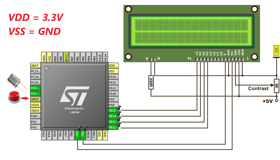
# 1. STM32单片机传感器接口概述**
STM32单片机集成了丰富的传感器接口,为开发人员提供了便捷的传感器连接和应用方案。传感器接口类型多样,包括模拟接口、数字接口和专用接口,满足不同传感器的连接需求。
通过传感器接口,STM32单片机可以获取传感器数据,进行数据处理和分析,从而实现各种应用功能。传感器接口的配置和使用涉及到硬件电路设计和软件编程,需要深入理解传感器特性和接口协议。
# 2.
程序哪里有错误 fun(int *p1,int *p2) { int *p; *p = *p1; *p1 = *p2; *p2 = *p; }
这个函数`fun(int *p1, int *p2)`存在几个错误和潜在问题:
1. 变量声明与赋值:你试图通过`*p = *p1`来分配指针`p`的值,但实际上`p`是一个未初始化的指针,直接赋值可能会导致不确定的行为。正确的做法是先为`p`指向一个内存位置。
2. 临时变量:你的代码没有明确使用`p`这个临时变量。如果你想交换`p1`和`p2`所指向的值,应该使用指针的解引用操作,而不是将`*p`赋值给它们。
3. 指向不确定的数据:由于`p`没有被初始化,如果它指向的是栈上的临时空间,当函数结束时这些值可能会丢失,除非特别指定它指向堆中的数据。
修复后的代码可能如下所示:
```
RFM2g接口驱动操作手册:API与命令行指南
本资源是《RFM2g Common Application Program Interface (API) 及 Command Line Interpreter for RFM2g Drivers》操作员参考手册,版本为Publication No. 523-000447-000 Rev. K.0。该文档详细介绍了RFM2g反射内存卡驱动程序的通用接口,这是一款专为提高系统性能和数据传输效率而设计的硬件设备。反射内存是一种高速、无主存访问延迟的技术,适用于对实时性有高要求的应用,如嵌入式系统和高性能计算环境。
文档内容涵盖了以下关键知识点:
1. **API接口**:手册提供了关于如何与RFM2g驱动进行交互的API指南,包括数据读写、配置、初始化和错误处理等接口函数的使用方法。用户可以根据这些API实现高效的数据通信,优化程序性能。
2. **Command Line Interpreter (CLI)**:手册还涉及一个命令行界面工具,允许用户通过命令行执行与驱动相关的操作,比如设置参数、监控状态和诊断问题,为调试和自动化流程提供了便利。
3. **文档历史**:修订版K.0更新于2016年9月,主要针对文档格式进行了调整,并强调了废物电气和电子设备(WEEE)管理,表明Abaco Systems遵循WEEE指令,对于2005年8月13日之前购买的产品,可能需要客户根据具体情况申请产品回收。
4. **安全警示**:手册中的警告、注意和提示部分,强调了安全操作的重要性,如避免可能导致人身伤害的危险行为(WARNING)、防止数据丢失或系统损坏的注意事项(CAUTION),以及提供有关功能特性和操作步骤的有用提示(TIP)。
5. **关于手册**:文档介绍了手册的使用规范和所用的通知类型,以确保用户在阅读和操作过程中能够理解和遵循相关指导。
这份文档是开发人员和系统管理员在使用RFM2g反射内存卡时的重要参考资料,提供了技术细节和最佳实践,有助于他们充分利用该硬件的特性来提升系统性能。对于从事嵌入式系统、实时数据处理或高性能计算领域的人来说,理解和掌握这个API和CLI是至关重要的。