揭秘MATLAB绘图中的坐标系与坐标变换：从二维到三维，轻松驾驭坐标世界

# 1. MATLAB绘图坐标系基础

MATLAB中绘图的坐标系是理解和创建图形的基础。本章将介绍MATLAB绘图中使用的各种坐标系，包括笛卡尔坐标系、极坐标系和三维坐标系。

### 笛卡尔坐标系

笛卡尔坐标系是最常用的坐标系，它使用两个垂直轴（x轴和y轴）来表示点的位置。x轴水平放置，y轴垂直放置。点的位置由其到x轴和y轴的距离表示，分别称为x坐标和y坐标。

% 创建一个笛卡尔坐标系
figure;
hold on;
plot([0 10], [0 10], 'r-'); % x轴
plot([0 10], [0 0], 'b-'); % y轴
xlabel('x');
ylabel('y');

# 2. 二维坐标系与变换

### 2.1 二维坐标系的定义和属性

#### 2.1.1 笛卡尔坐标系

笛卡尔坐标系是一种二维坐标系，它由两条互相垂直的直线轴组成，分别称为 x 轴和 y 轴。坐标系原点是两条轴的交点，表示 (0, 0) 点。

任何一个点在笛卡尔坐标系中的位置都可以用一对有序数 (x, y) 来表示，其中 x 表示点到 y 轴的距离，y 表示点到 x 轴的距离。

#### 2.1.2 极坐标系

极坐标系也是一种二维坐标系，它由一个原点和一条从原点出发的射线组成。射线称为极轴，原点称为极点。

任何一个点在极坐标系中的位置可以用一对有序数 (r, θ) 来表示，其中 r 表示点到极点的距离，θ 表示极轴与点到极点的连线之间的夹角。

### 2.2 二维坐标系的变换

二维坐标系变换是指将一个坐标系中的点转换到另一个坐标系中的过程。常见的二维坐标系变换包括平移变换、旋转变换和缩放变换。

#### 2.2.1 平移变换

平移变换是指将坐标系中的所有点沿一个向量平移。平移向量的分量表示平移的距离和方向。

% 平移变换示例
x = [1, 2, 3];
y = [4, 5, 6];

% 平移向量
dx = 2;
dy = 3;

% 平移变换
x_new = x + dx;
y_new = y + dy;

**逻辑分析：**

* `x` 和 `y` 数组分别表示原始坐标系中的 x 坐标和 y 坐标。
* `dx` 和 `dy` 分别表示平移向量的 x 分量和 y 分量。
* `x_new` 和 `y_new` 数组分别表示平移后的 x 坐标和 y 坐标。

#### 2.2.2 旋转变换

旋转变换是指将坐标系中的所有点绕一个固定点旋转一个角度。旋转点称为旋转中心，旋转角度称为旋转角。

% 旋转变换示例
x = [1, 2, 3];
y = [4, 5, 6];

% 旋转中心
cx = 2;
cy = 3;

% 旋转角度（弧度）
theta = pi/4;

% 旋转变换
x_new = (x - cx) * cos(theta) - (y - cy) * sin(theta) + cx;
y_new = (x - cx) * sin(theta) + (y - cy) * cos(theta) + cy;

**逻辑分析：**

* `x` 和 `y` 数组分别表示原始坐标系中的 x 坐标和 y 坐标。
* `cx` 和 `cy` 分别表示旋转中心的 x 坐标和 y 坐标。
* `theta` 表示旋转角度，以弧度为单位。
* `x_new` 和 `y_new` 数组分别表示旋转后的 x 坐标和 y 坐标。

#### 2.2.3 缩放变换

缩放变换是指将坐标系中的所有点沿 x 轴和 y 轴分别缩放一个比例因子。缩放因子称为缩放比例。

% 缩放变换示例
x = [1, 2, 3];
y = [4, 5, 6];

% 缩放比例
sx = 2;
sy = 3;

% 缩放变换
x_new = x * sx;
y_new = y * sy;

**逻辑分析：**

* `x` 和 `y` 数组分别表示原始坐标系中的 x 坐标和 y 坐标。
* `sx` 和 `sy` 分别表示 x 轴和 y 轴的缩放比例。
* `x_new` 和 `y_new` 数组分别表示缩放后的 x 坐标和 y 坐标。

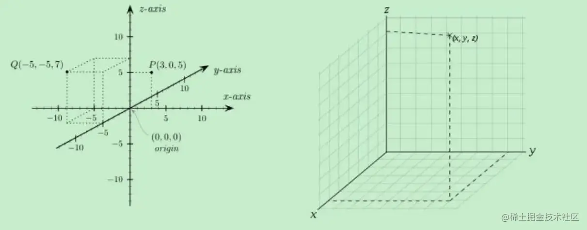
# 3.1 三维坐标系的定义和属性

### 3.1.1 直角坐标系

三维直角坐标系由三个相互垂直的坐标轴组成，分别表示 x、y 和 z 轴。每个轴表示一个空间维度，并且它们在原点处相交。

**定义：**

[x, y, z] = (x, y, z)

**属性：**

* **原点：**坐标轴相交的点，表示所有坐标为零的点。
* **坐标平面：**由两个坐标轴形成的平面，例如 xy 平面、yz 平面和 xz 平面。
* **八分仪：**将空间划分为八个象限的三个坐标平面。

### 3.1.2 柱面坐标系

柱面坐标系由三个坐标表示：

* **径向坐标 (r)：**从原点到点的距离。
* **方位角 (θ)：**从 x 轴正方向到 r 矢量的逆时针角度。
* **高度坐标 (z)：**点在 z 轴上的高度。

**定义：**

[r, θ, z] = (r, θ, z)

**属性：**

* **原点：**坐标轴相交的点，表示所有坐标为零的点。
* **基平面：**由 xy 平面形成的平面。
* **柱面：**由 r 和 θ 坐标形成的曲面。

### 3.1.3 球面坐标系

球面坐标系由三个坐标表示：

* **径向坐标 (r)：**从原点到点的距离。
* **仰角 (φ)：**从 z 轴正方向到 r 矢量的逆时针角度。
* **方位角 (θ)：**从 x 轴正方向到 r 矢量在 xy 平面上的投影的逆时针角度。

**定义：**

[r, φ, θ] = (r, φ, θ)

**属性：**

* **原点：**坐标轴相交的点，表示所有坐标为零的点。
* **基平面：**由 xy 平面形成的平面。
* **球面：**由 r、φ 和 θ 坐标形成的曲面。

# 4. 坐标系变换的实践应用

### 4.1 图形绘制中的坐标系变换

坐标系变换在图形绘制中扮演着至关重要的角色，它允许我们对图形进行平移、旋转和缩放等操作，从而实现更灵活的图形绘制。

#### 4.1.1 二维图形的坐标系变换

在二维图形绘制中，坐标系变换主要用于以下场景：

- **平移变换：**将图形沿 x 轴或 y 轴平移一定距离。
- **旋转变换：**将图形绕原点旋转一定角度。
- **缩放变换：**将图形沿 x 轴或 y 轴缩放一定倍数。

% 二维图形平移变换
figure;
plot([1, 2, 3], [4, 5, 6]);
title('平移前');
xlabel('x');
ylabel('y');

% 平移图形
translation_vector = [2, 1];
translated_points = [1, 2, 3] + translation_vector(1);
translated_points = [4, 5, 6] + translation_vector(2);
hold on;
plot(translated_points, translated_points, 'r');
title('平移后');
legend('平移前', '平移后');

% 二维图形旋转变换
figure;
plot([1, 2, 3], [4, 5, 6]);
title('旋转前');
xlabel('x');
ylabel('y');

% 旋转图形
rotation_angle = pi / 4;
rotation_matrix = [cos(rotation_angle), -sin(rotation_angle); sin(rotation_angle), cos(rotation_angle)];
rotated_points = rotation_matrix * [1, 2, 3; 4, 5, 6]';
hold on;
plot(rotated_points(1, :), rotated_points(2, :), 'r');
title('旋转后');
legend('旋转前', '旋转后');

% 二维图形缩放变换
figure;
plot([1, 2, 3], [4, 5, 6]);
title('缩放前');
xlabel('x');
ylabel('y');

% 缩放图形
scale_factor = 2;
scaled_points = scale_factor * [1, 2, 3; 4, 5, 6];
hold on;
plot(scaled_points(1, :), scaled_points(2, :), 'r');
title('缩放后');
legend('缩放前', '缩放后');

#### 4.1.2 三维图形的坐标系变换

在三维图形绘制中，坐标系变换的应用更加广泛，除了平移、旋转和缩放变换外，还包括透视投影等高级变换。

% 三维图形平移变换
figure;
plot3([1, 2, 3], [4, 5, 6], [7, 8, 9]);
title('平移前');
xlabel('x');
ylabel('y');
zlabel('z');

% 平移图形
translation_vector = [2, 1, 3];
translated_points = [1, 2, 3] + translation_vector(1);
translated_points = [4, 5, 6] + translation_vector(2);
translated_points = [7, 8, 9] + translation_vector(3);
hold on;
plot3(translated_points, translated_points, translated_points, 'r');
title('平移后');
legend('平移前', '平移后');

% 三维图形旋转变换
figure;
plot3([1, 2, 3], [4, 5, 6], [7, 8, 9]);
title('旋转前');
xlabel('x');
ylabel('y');
zlabel('z');

% 旋转图形
rotation_angle = pi / 4;
rotation_matrix = [cos(rotation_angle), -sin(rotation_angle), 0; sin(rotation_angle), cos(rotation_angle), 0; 0, 0, 1];
rotated_points = rotation_matrix * [1, 2, 3; 4, 5, 6; 7, 8, 9]';
hold on;
plot3(rotated_points(1, :), rotated_points(2, :), rotated_points(3, :), 'r');
title('旋转后');
legend('旋转前', '旋转后');

% 三维图形缩放变换
figure;
plot3([1, 2, 3], [4, 5, 6], [7, 8, 9]);
title('缩放前');
xlabel('x');
ylabel('y');
zlabel('z');

% 缩放图形
scale_factor = 2;
scaled_points = scale_factor * [1, 2, 3; 4, 5, 6; 7, 8, 9];
hold on;
plot3(scaled_points(1, :), scaled_points(2, :), scaled_points(3, :), 'r');
title('缩放后');
legend('缩放前', '缩放后');

### 4.2 数据可视化中的坐标系变换

坐标系变换在数据可视化中也发挥着重要作用，它可以帮助我们从不同角度观察数据，发现隐藏的规律。

#### 4.2.1 二维数据的可视化

在二维数据可视化中，坐标系变换主要用于以下场景：

- **散点图变换：**将散点图中的数据点沿 x 轴或 y 轴平移、旋转或缩放，以突出显示数据之间的关系。
- **条形图变换：**将条形图中的条形沿 x 轴或 y 轴平移、旋转或缩放，以比较不同组别的数据。
- **饼图变换：**将饼图中的扇形沿圆心平移、旋转或缩放，以强调不同类别的数据占比。

% 二维数据可视化中的散点图变换
figure;
scatter(randn(100, 1), randn(100, 1));
title('散点图变换前');
xlabel('x');
ylabel('y');

% 平移散点图
translation_vector = [2, 1];
translated_data = randn(100, 1) + translation_vector(1);
translated_data = randn(100, 1) + translation_vector(2);
hold on;
scatter(translated_data, translated_data, 'r');
title('散点图变换后');
legend('变换前', '变换后');

% 二维数据可视化中的条形图变换
figure;
bar([1, 2, 3], [4, 5, 6]);
title('条形图变换前');
xlabel('x');
ylabel('y');

% 平移条形图
translation_vector = [2, 1];
translated_data = [1, 2, 3] + translation_vector(1);
translated_data = [4, 5, 6] + translation_vector(2);
hold on;
bar(translated_data, translated_data, 'r');
title('条形图变换后');
legend('变换前', '变换后');

% 二维数据可视化中的饼图变换
figure;
pie([1, 2, 3]);
title('饼图变换前');

% 旋转饼图
rotation_angle = pi / 4;
rotated_data = [cos(rotation_angle), -sin(rotation_angle); sin(rotation_angle), cos(rotation_angle)] * [1, 2, 3]';
hold on;
pie(rotated_data, 'r');
title('饼图变换后');
legend('变换前', '变换后');

#### 4.2.2 三维数据的可视化

在三维数据可视化中，坐标系变换的应用更加广泛，除了平移、旋转和缩放变换外，还包括透视投影等高级变换。

% 三维数据可视化中的散点图变换
figure;
scatter3(randn(100, 1), randn(100, 1), randn(100, 1));
title('三维散点图变换前');
xlabel('x');
ylabel('y');
zlabel('z');

% 平移三维散点图
translation_vector = [2, 1, 3];
translated_data = randn(100, 1) + translation_vector(1);
translated_data = randn(100, 1) + translation_vector(2);
translated_data = randn(100, 1) + translation_vector(3);
hold on;
scatter3(translated

# 5. MATLAB绘图中的坐标系与变换高级技巧

### 5.1 坐标系自定义

#### 5.1.1 自定义坐标系轴

在MATLAB中，可以使用`axis`函数自定义坐标系轴。`axis`函数的参数可以指定坐标轴的范围、刻度和标签。

% 设置x轴范围为[0, 10]，y轴范围为[-5, 5]
axis([0 10 -5 5]);

% 设置x轴刻度为1，y轴刻度为2
axis([0 10 -5 5], 'xTick', 0:1:10, 'yTick', -5:2:5);

% 设置x轴标签为'时间(s)'，y轴标签为'幅度'
xlabel('时间(s)');
ylabel('幅度');

#### 5.1.2 自定义坐标系标签

可以使用`xlabel`和`ylabel`函数自定义坐标系标签。

% 设置x轴标签为'时间(s)'
xlabel('时间(s)');

% 设置y轴标签为'幅度'
ylabel('幅度');

### 5.2 坐标系交互

#### 5.2.1 坐标系缩放和平移

可以使用`zoom`和`pan`函数进行坐标系缩放和平移。

% 缩放坐标系
zoom(2);

% 平移坐标系
pan(10, 20);

#### 5.2.2 坐标系旋转

可以使用`view`函数旋转坐标系。

% 将坐标系旋转30度
view(30, 30);