
Unsupervised Anomaly Detection via Variational Auto-Encoder
for Seasonal KPIs in Web Applications WWW 2018, April 23–27, 2018, Lyon, France
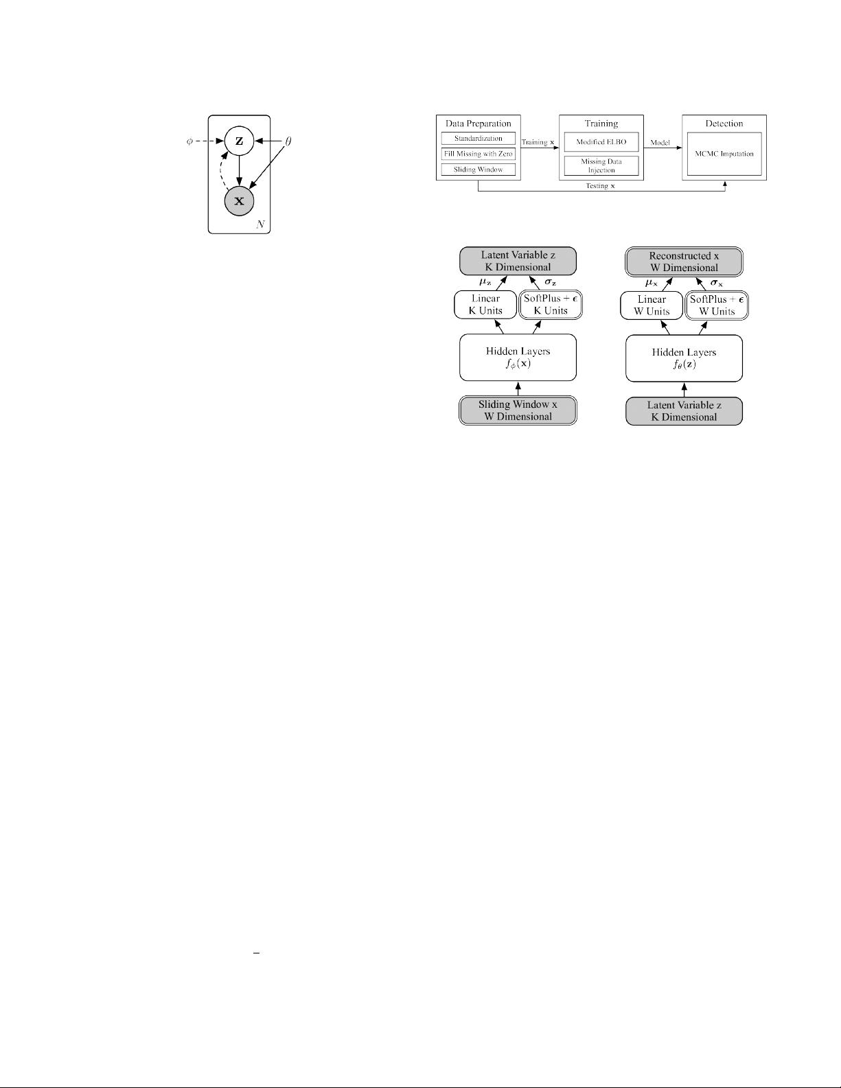
Figure 2: Architecture of VAE. The prior of z is regarded as
part of the generative model (solid lines), thus the whole
generative model is denoted as p
θ
(x, z) = p
θ
(x|z)p
θ
(z). The
approximated posterior (dashed lines) is denoted as q
ϕ
(z|x).
2.4 Background of Variational Auto-Encoder
Deep Bayesian networks use neural networks to express the rela-
tionships between variables, such that they are no longer restricted
to simple distribution families, thus can be easily applied to compli-
cated data. Variational inference techniques [
12
] are often adopted
in training and prediction, which are ecient methods to solve
posteriors of the distributions derived by neural networks.
VAE is a deep Bayesian network. It models the relationship be-
tween two random variables, latent variable
z
and visible vari-
able
x
. A prior is chosen for
z
, which is usually multivariate unit
Gaussian
N(0, I)
. After that,
x
is sampled from
p
θ
(x|z)
, which is
derived from a neural network with parameter
θ
. The exact form
of
p
θ
(x|z)
is chosen according to the demand of task. The true pos-
terior
p
θ
(z|x)
is intractable by analytic methods, but is necessary
for training and often useful in prediction, thus the variational
inference techniques are used to t another neural network as
the approximation posterior
q
ϕ
(z|x)
. This posterior is usually as-
sumed to be
N(µ
ϕ
(x), σ
2
ϕ
(x))
, where
µ
ϕ
(x)
and
σ
ϕ
(x)
are derived
by neural networks. The architecture of VAE is shown as Fig 2.
SGVB [
16
,
32
] is a variational inference algorithm that is often
used along with VAE, where the approximated posterior and the
generative model are jointly trained by maximizing the evidence
lower bound (ELBO, Eqn (1)). We did not adopt more advanced
variational inference algorithms, since SGVB already works.
logp
θ
(x) ≥ log p
θ
(x) − KL
q
ϕ
(z|x)
p
θ
(z|x)
= L(x) (1)
= E
q
ϕ
(z |x)
logp
θ
(x) + log p
θ
(z|x) − log q
ϕ
(z|x)
= E
q
ϕ
(z |x)
logp
θ
(x, z) − log q
ϕ
(z|x)
= E
q
ϕ
(z |x)
logp
θ
(x|z) + logp
θ
(z) − log q
ϕ
(z|x)
Monte Carlo integration [
10
] is often adopted to approximate the
expectation in Eqn (1), as Eqn (2), where
z
(l)
, l =
1
. . . L
are samples
from q
ϕ
(z|x). We stick to this method throughout this paper.
E
q
ϕ
(z |x)
[
f (z)
]
≈
1
L
L
Õ
l=1
f (z
(l)
) (2)
Figure 3: Overall architecture of Donut.
(a) Variational net q
ϕ
(z |x) (b) Generative net p
θ
(x |z)
Figure 4: Network structure of Donut. Gray nodes are ran-
dom variables, and white nodes are layers. The double lines
highlight our special designs upon a general VAE.
3 ARCHITECTURE
The overall architecture of our algorithm Donut is illustrated as
Fig 3. The three key techniques are Modied ELBO and Missing
Data Injection during training, and MCMC Imputation in detection.
3.1 Network Structure
As aforementioned in
§
2.1, the KPIs studied in this paper are
assumed to be time sequences with Gaussian noises. However, VAE
is not a sequential model, thus we apply sliding windows [
34
] of
length
W
over the KPIs: for each point
x
t
, we use
x
t −W +1
, . . . , x
t
as
the
x
vector of VAE. This sliding window was rst adopted because
of its simplicity, but it turns out to actually bring an important and
benecial consequence, which will be discussed in § 5.1.
The overall network structure of Donut is illustrated in Fig 4,
where the components with double-lined outlines (e.g., Sliding Win-
dow x, W Dimensional at bottom left) are our new designs and the
remaining components are from standard VAEs. The prior
p
θ
(z)
is
chosen to be N(0, I). Both x and z posterior are chosen to be diag-
onal Gaussian:
p
θ
(x|z) = N (µ
x
, σ
x
2
I)
, and
q
ϕ
(z|x) = N (µ
z
, σ
z
2
I)
,
where
µ
x
,
µ
z
and
σ
x
,
σ
z
are the means and standard deviations of
each independent Gaussian component.
z
is chosen to be
K
dimen-
sional. Hidden features are extracted from
x
and
z
, by separated
hidden layers
f
ϕ
(x)
and
f
θ
(z)
. Gaussian parameters of
x
and
z
are
then derived from the hidden features. The means are derived from
linear layers:
µ
x
= W
⊤
µ
x
f
θ
(z) + b
µ
x
and
µ
z
= W
⊤
µ
z
f
ϕ
(x) + b
µ
z
.
The standard deviations are derived from soft-plus layers, plus a
non-negative small number
ϵ
:
σ
x
= SoPlus[W
⊤
σ
x
f
θ
(z) + b
σ
x
] + ϵ
and
σ
z
= SoPlus[W
⊤
σ
z
f
ϕ
(x) + b
σ
z
] + ϵ
, where
SoPlus[a] =
剩余11页未读,继续阅读

weixin_38550722
- 粉丝: 8
- 资源: 928
 我的内容管理
展开
我的内容管理
展开


最新资源
- OptiX传输试题与SDH基础知识
- C++Builder函数详解与应用
- Linux shell (bash) 文件与字符串比较运算符详解
- Adam Gawne-Cain解读英文版WKT格式与常见投影标准
- dos命令详解:基础操作与网络测试必备
- Windows 蓝屏代码解析与处理指南
- PSoC CY8C24533在电动自行车控制器设计中的应用
- PHP整合FCKeditor网页编辑器教程
- Java Swing计算器源码示例:初学者入门教程
- Eclipse平台上的可视化开发:使用VEP与SWT
- 软件工程CASE工具实践指南
- AIX LVM详解:网络存储架构与管理
- 递归算法解析:文件系统、XML与树图
- 使用Struts2与MySQL构建Web登录验证教程
- PHP5 CLI模式:用PHP编写Shell脚本教程
- MyBatis与Spring完美整合:1.0.0-RC3详解
资源上传下载、课程学习等过程中有任何疑问或建议,欢迎提出宝贵意见哦~我们会及时处理!
点击此处反馈


