ñ⁺
m ⁺
v
w ⁺
w ⁻
m ⁻
ñ⁻
narrow interval
rounding interval
wide interval
uncovered intervals
v ⁺
v ⁻
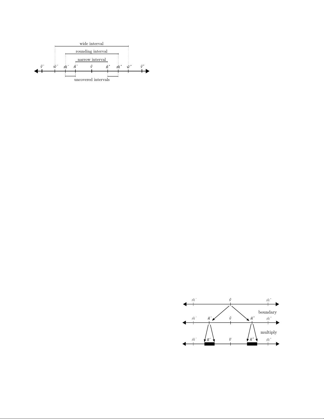
Figure 1: Representations, Midpoints and Boundaries: ˆv denotes a
native, machine representable floating point number with neighbors
ˆv
−
and ˆv
+
; ˜m
−
and ˜m
+
denote exact midpoints; ˜n
−
and ˜n
+
denote the narrow (or conservative) boundaries; ˜w
−
and ˜w
+
denote
wide boundaries; and the uncovered intervals denote the portion of
the rounding interval not covered by the narrow interval.
•
Step 1: Compute narrow boundaries ˜n
−
, ˜n
+
such that:
˜m
−
< ˜n
−
< ˆv < ˜n
+
< ˜m
+
•
Step 2: Compute shortest decimal in the interval [˜n
−
, ˜n
+
].
By relaxing the constraints of using exact midpoints ˜m
−
, ˜m
+
,
Grisu3 can use efficient operations over limited-precision numbers
(instead of Dragon4’s bignum) to yield provably correct albeit
possibly suboptimal conversions.
Scaled Narrow Intervals. A triple (e, ¯n
−
, ¯n
+
) is a scaled narrow
interval for ˆv if there exists ˜n
−
, ˜n
+
such that:
1. ¯n
+
∈ (1, 10]
2. ¯n
−
≈ 10
−e
× ˜n
−
3. ¯n
+
≈ 10
−e
× ˜n
+
4. ˜m
−
< ˜n
−
< ˆv < ˜n
+
< ˜m
+
Intuitively, a scaled narrow interval for ˆv corresponds to a narrow
interval for ˆv where the boundaries are scaled by 10
−e
to ensure
that the upper bound ¯n
+
is in (1, 10]. Note that the last requirement
allows us to compute the (scaled) narrow intervals approximately,
e.g. using HP numbers, as long as the (unscaled) boundaries reside
within the exact midpoints ˜m
−
and ˜m
+
. Finally, only the upper
boundary ¯n
+
must be in the interval (1, 10], hence we observe that
the exponent is e ≈ blog
10
˜n
+
c.
Algorithm. Figure 2 formalizes the above intuition in a generic
algorithm to convert an input FP value ˆv into decimal form
comprising a pair of a sequence of digits d
1
, . . . , d
N
and an ex-
ponent e denoting the decimal value 0.d
1
. . . d
N
× 10
e
. (Although
this differs slightly from the normal format – with a leading non-
zero digit – we can normalize by shifting the decimal point to
the right.) The convert algorithm is split into two procedures,
narrow_interval and digits, corresponding to the steps de-
scribed above. The first phase narrow_interval begins with
the input ˆv and computes a scaled narrow interval (e, ¯n
−
, ¯n
+
) for
ˆv. The second phase digits uses the scaled narrow interval to
compute the final output digits corresponding to the shortest dec-
imal value within the scaled narrow interval [¯n
−
, ¯n
+
]. Next, we
describe the two steps in detail.
3.2 Step 1: Compute Narrow Interval
The first phase computes the scaled narrow interval (e, ¯n
−
, ¯n
+
)
for the input ˆv. First, the (unscaled) boundary ˜n
−
, ˜n
+
is computed
directly from the input ˆv by the function boundary. Second, the
exponent e is directly computed from the upper boundary ˜n
+
by
scaling it to ensure that its significand lies in the range [1, 10). That
def convert(ˆv):
(e,¯n
−
,¯n
+
) = narrow_interval(ˆv)
digits = digits(¯n
−
,¯n
+
)
return (digits,e)
def narrow_interval(ˆv):
(˜n
−
,˜n
+
) = boundary(ˆv)
e = floor(log10(˜n
+
))
¯n
−
= multiply(˜n
−
, 10
−e
)
¯n
+
= multiply(˜n
+
, 10
−e
)
return (e,¯n
−
,¯n
+
)
def digits(¯n
−
,¯n
+
):
digits = []
repeat:
(¯n
−
,d
−
) = next_digit(¯n
−
)
(¯n
+
,d
+
) = next_digit(¯n
+
)
digits.append(d
+
)
until(d
−
!= d
+
)
return digits
def next_digit(¯n):
d = truncate(¯n)
¯n = multiply(¯n - d, 10)
return (¯n,d)
Figure 2: A Generic Conversion Algorithm
is, the exponent e is computed as the value blog
10
˜n
+
c. Finally,
using the exponent, the scaled narrow boundaries are computed by
multiplying the narrow boundaries by 10
−e
.
The functions boundary and multiply are deliberately left
abstract. However, any concrete implementations must take care to
ensure that despite errors introduced by rounding and propagation,
the overall output is indeed a valid narrow interval for ˆv. Conse-
quently, the narrow boundaries computed by boundary are cho-
sen in a conservative fashion – as shown in Figure 3 – so that de-
spite any rounding and propagation errors, the results remain within
the actual midpoints, and hence form a valid narrow interval.
m ⁻
m ⁺
v
m ⁻
m ⁺
v
ñ⁺
ñ⁻
boundary
m ⁻
m ⁺
v n
⁺
n ⁻
multiply
Figure 3: Error Propagation. The multiply operation computes the
scaled interval (¯n
−
, ¯n
+
) with error (as represented by the black
boxes), creating the requirement that the narrow interval (˜n
−
, ˜n
+
)
be conservative enough to prevent overlap with the scaled mid-
points ¯m
−
and ¯m
+


