深度学习高效处理教程：架构与技术综览

需积分: 50 2 浏览量更新于2024-07-17 收藏 5.13MB PDF 举报

本文档深入探讨了"Efficient Processing of Deep Neural Networks: A Tutorial and Survey"，它作为深度学习领域的重要参考资料，提供了对自本世纪初以来深度学习技术迅猛发展及其在硬件加速方面的最新进展进行全面的概述。深度神经网络（DNNs）凭借其在计算机视觉、语音识别和机器人技术等人工智能应用中的卓越性能，已成为行业的标准。然而，其高度计算复杂性使得能源效率和吞吐量的提升成为亟待解决的问题，同时还需要维持或提高性能准确性和控制硬件成本。文章首先介绍了深度神经网络的基本概念和原理，强调了在AI系统中广泛应用DNNs所面临的挑战，即如何在保持高性能的同时实现计算效率的提升。接下来，作者详细梳理了各类支持DNN的平台和架构，包括云端服务器、嵌入式设备、专用硬件如GPU和TPU，以及FPGA和ASIC等，这些硬件的不同特性决定了它们在处理深度学习任务时的优势和局限性。重点部分深入讨论了近期在提高DNN效率方面的主要技术趋势。这包括但不限于： 1. **模型优化**：通过对神经网络结构进行剪枝、量化和蒸馏，降低模型的参数数量和计算复杂度，从而减少运算需求，提高执行速度。 2. **硬件加速**：通过硬件设计的专门化，如GPU的并行计算能力、TPU的矩阵运算优化，以及定制芯片（ASIC）的低延迟和高能效，来加速深度学习任务的处理。 3. **近似计算**：利用近似计算和低精度计算技术，允许在一定程度上牺牲精确度以换取更高的性能，这对于实时应用和移动设备尤其关键。 4. **硬件-software协同**：通过软件层面的优化，如数据预处理、模型编译和硬件调度策略，以及硬件和软件之间的协同工作，来进一步提升整体效率。 5. **动态调度和适应性**：通过动态调整网络执行策略，根据任务需求和硬件资源实时改变计算负载，实现资源的高效利用。 6. **可扩展性和灵活性**：研究如何在不同的硬件环境下实现深度学习模型的无缝迁移，以适应不同场景的需求。这篇文章是一份宝贵的指南，对于研究人员、工程师和开发者来说，它不仅提供了深度学习基础的回顾，还提供了关于如何在实际应用中实现高效处理DNNs的实用策略和趋势分析，为推动AI系统的广泛应用和发展奠定了坚实的基础。

the output. In these networks, some intermediate operations

generate values that are stored internally to the network and

used as inputs to other operations in conjunction with the

processing of a later input. In this article, we will focus on

feed-forward networks as to-date little attention has been given

to hardware acceleration speciﬁcally of recurrent networks.

DNNs can be composed of fully-connected (FC, also referred

to as multi-layer perceptrons) as shown in the leftmost layer

of Fig. 2(d). In a fully-connected layer, all output activations

are composed of a weighted sum of all input activations

(i.e., all outputs are connected to all inputs). This requires a

signiﬁcant amount of storage and computation. Thankfully, in

many applications, we can remove some connections between

the activations by setting the weights to zero without affecting

accuracy. This results in a sparsely-connected layer. A sparsely

connected layer is illustrated in the rightmost layer of Fig. 2(d).

We can also make the computation more efﬁcient by limiting

the number of weights that contribute to an output. This sort of

structured sparsity can arise if each output is only a function

of a ﬁxed-size window of inputs. Even further efﬁciency can

be gained if the same set of weights are used in the calculation

of every output. This weight sharing can signiﬁcantly reduce

the storage requirements for weights.

An extremely popular windowed, weight-shared network

arises by structuring the computation as a convolution, as

shown in Fig. 6(a), where the output is computed using only

a small neighborhood of activations for the weighted sum (i.e.,

the ﬁlter has a limited receptive ﬁeld, and all weights beyond

a certain distance from the input is set to zero), and where

the same set of weights are shared for every output (i.e., the

ﬁlter is space invariant). This is a form of structured sparsity

is orthogonal to the sparsity that occurs from network pruning

as described in Section

VII-B

2. Accordingly, a convolutional

neural network (CNN) is a popular form of DNN [35].

1) Convolutional Neural Networks (CNNs): CNNs are

composed of multiple convolutional layers (CONV), as shown

in Fig. 7, where each layer generates a higher-level abstraction

of the input data, called a feature map (fmap), that preserves

essential yet unique information. Modern CNNs are able

to achieve superior performance by employing a very deep

hierarchy of layers. CNN, also known as ConvNets, are

widely used in a variety of applications including image

understanding [

], speech recognition [

], game play [

robotics [

], etc. The paper will focus on its use in image

processing, speciﬁcally for the task of image classiﬁcation [

Each of the CONV layers in the CNN is primarily composed

of high-dimensional convolutions as shown in Fig. 6(b). In this

computation there are a set of 2-D input feature maps (ifmaps),

each of which is called a channel. Each channel is convolved

with a distinct 2-D ﬁlter from the stack of ﬁlters, one for

each channel. The results of the convolution at each point are

summed across all the channels. In addition, a 1-D bias can be

added to the ﬁltering results, but some recent networks [

]

remove its usage from part of the layers. The result of this

computation is one channel of output feature map (ofmap).

Additional stacks of 2-D ﬁlters can be used on the same input

to create additional output channels. Finally, multiple stacks

of input feature maps may be processed together as a batch to

filter (weights)

Partial Sum (psum)

Accumulation

input fmap output fmap

Element-wise

Multiplication

an output

activation

(a) 2-D convolution in traditional image processing

Input fmaps

Filters

Output fmaps

…

(b) High dimensional convolutions in CNNs

Fig. 6. Dimensionality of convolutions.

Modern Deep CNN: 5 – 1000 Layers

Class

Scores

Layer

CONV

Layer

Low-Level

Features

CONV

Layer

High-Level

Features

…

1 – 3 Layers

Convolu'on(

Non-linearity(

×(

Normaliza'on(

Pooling(

Optional

Fully(

Connected(

×(

Non-linearity(

CONV

Layer

Mid-Level

Features

Fig. 7. Convolutional Neural Networks.

potentially improve reuse of the ﬁlter weights.

Given the shape parameters in Table I, the computation of

a CONV layer is deﬁned as

O[z][u][x][y] = B[u] +

C−1

k=0

R−1

i=0

R−1

j=0

I[z][k][Ux + i][Uy + j] × W[u][k][i][j],

0 ≤ z < N, 0 ≤ u < M, 0 ≤ x, y < E, E = (H − R + U)/U.

(1)

and

are the matrices of the ofmaps, ifmaps, ﬁlters

and biases, respectively.

is a given stride size. Fig. 6(b)

shows a visualization of this computation (ignoring biases).

To align the terminology of CNNs with the generic DNN,

• ﬁlters are composed of weights (i.e., synapses)

• input images are composed of pixels (i.e., input neurons

to ﬁrst layer)

•

input and output feature maps (ifmaps, ofmaps) are

composed of activations (i.e., input and output neurons)

Shape Parameter Description

N batch size of 3-D fmaps

M # of 3-D ﬁlters / # of ofmap channels

C # of ifmap/ﬁlter channels

H ifmap plane width/height

R ﬁlter plane width/height (= H in FC)

E ofmap plane width/height (= 1 in FC)

TABLE I

SHAPE PARAMETERS OF A CONV/FC LAYER.

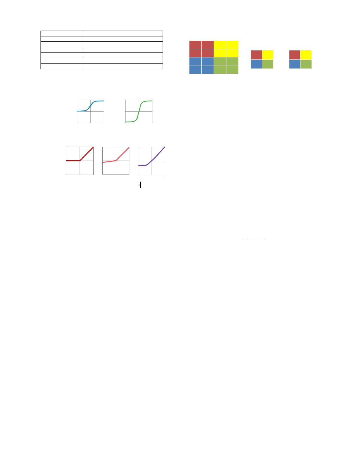
Sigmoid

-1

0 1

-1

!"#$%#&'

()

Hyperbolic Tangent

-1

0 1

-1

!"%'

)

()

*$%'

)

()

Rectified Linear Unit

(ReLU)

-1

0 1

-1

!",-)%./)*+

Leaky ReLU

-1

0 1

-1

!",-)%0)/)*+

Exponential LU

-1

0 1

-1

++++)/+++++++

++++0%'

)

(#*/+

)1.+

)2.+

!"+

α = small const. (e.g. 0.1)

Traditional

Non-Linear

Activation

Functions

Modern

Non-Linear

Activation

Functions

Fig. 8. Various forms of non-linear activation functions (Figure adopted from

Caffe Tutorial [43]).

From ﬁve [

] to even more than a thousand [

] CONV

layers are commonly used in recent CNN models. A small

number, e.g., 1 to 3, of fully-connected (FC) layers are typically

applied after the CONV layers for classiﬁcation purposes. A FC

layer also applies ﬁlters on the ifmaps as in the CONV layers,

but the ﬁlters are of the same size as the ifmaps. Therefore,

it does not have the weight sharing property of CONV layers.

Eq. (1) still holds for the computation of FC layers with a

few additional constraints on the shape parameters:

H = R

E = 1, and U = 1.

In addition to CONV and FC layers, various optional layers

can be found in a DNN such as the non-linearity (NON),

pooling (POOL), and normalization (NORM). Each of these

layers can be conﬁgured as discussed next.

2) Non-Linearity: A non-linear activation function is typ-

ically applied after each convolution or fully connected

computation. Various non-linear functions are used to introduce

non-linearity into the DNN as shown in Fig. 8. These include

conventional non-linear functions such as sigmoid or hyperbolic

tangent as well as rectiﬁed linear unit (ReLU) [

], which has

become popular in recent years due to its simplicity and its

ability to enable fast training. Variations of ReLU, such as leaky

ReLU [

], parametric ReLU [

], and exponential LU [

]

have also been explored for improved accuracy. Finally, a

non-linearity called maxout, which takes the max value of

two intersecting linear functions, has shown to be effective in

speech recognition tasks [41, 42].

3) Pooling: Pooling enables the network to be robust and

invariant to small shifts and distortions and is applied to each

channel separately. It can be conﬁgured based on the size of

9 3 5 3

10 32 2 2

1 3 21 9

2 6 11 7

2x2 pooling, stride 2

32 5

6 21

Max pooling

Average pooling

18 3

3 12

Fig. 9. Various forms of pooling (Figure adopted from Caffe Tutorial [

]).

its receptive ﬁeld (e.g., 2

2) and the type of pooling (e.g.,

max or average), as shown in Fig. 9. Typically the pooling

occurs on non-overlapping blocks (i.e., the stride is equal to

the size of the pooling). Usually a stride of greater than one

is used such that there is a reduction in the dimension of the

representation (i.e., feature map).

4) Normalization: Controlling the input distribution across

layers can help to signiﬁcantly speed up training and improve

accuracy. Accordingly, the distribution of the layer input

activations (

) are normalized such that it has a zero mean

and a unit standard deviation. In batch normalization, the

normalized value is further scaled and shifted, as shown in

Eq. (2), the parameters (

) are learned from training [



is a small constant to avoid numerical problems. Prior to this,

local response normalization [

] was used, which was inspired

by lateral inhibition in neurobiology where excited neurons

(i.e., high values activations) should subdue its neighbors (i.e.,

low value activations); however, batch normalization is now

considered standard practice in the design of CNNs.

y =

x − µ

√

+ 

γ + β

(2)

A. Popular DNN Models

Many DNN models have been developed over the past

two decades. Each of these models has a different ”network

architecture” in terms of number of layers, ﬁlter shapes (i.e.,

ﬁlter size, number of channels and ﬁlters), layer types, and

connections between layers. Understanding these variations

and trends is important for incorporating the right ﬂexibility

in any efﬁcient DNN engine.

Although the ﬁrst popular DNN, LeNet [

], was published

in the 1990s, it wasn’t until 2012 that the AlexNet [

] was

used in the ImageNet Challenge [

]. We will give an overview

of various popular DNNs that competed in and/or won the

ImageNet Challenge [

] as shown in Fig. 5, most of whose

models with pre-trained weights are publicly available for

download; the DNN models are summarized in Table II. Two

results for top-5 error results are reported. In the ﬁrst row, the

accuracy is boosted by using multiple crops from the image,

and an ensemble of multiple trained models (i.e., the DNN

needs to be run several times); these are results that are used to

compete in the ImageNet Challenge. The second row reports

the accuracy if only a single crop was used (i.e., the DNN is

run only once), which is more consistent with what would be

deployed in real applications.

LeNet [9] was one of the ﬁrst CNN approaches introduced

in 1989. It was designed for the task of digit classiﬁcation

in grayscale images of size 28

28. The most well known

剩余30页未读，继续阅读

Dongxu_Lv

粉丝: 1507
资源: 5

深度学习高效处理教程：架构与技术综览

"深度学习框架下的单事件视频描述方法研究:人工智能视觉与自然语言结合的新进展

"优化快速神经网络计算方法：卷积定理与点积方法对比研究"。

深度学习基础及卷积神经网络应用详解

Efficient Processing of Deep Neural Networks: A Tutorial and Survey

深度学习国外综述论文 Efficient Processing of Deep Neural Networks: A Tutorial and Survey

efficient processing of deep neural networks

efficient processing of deep neural networks pdf

Hyperbolic Deep Neural Networks A Survey.zip

Hyperbolic Deep Neural Networks A Survey.pdf

Video Summarization Using Deep Neural Networks A Survey.zip

最新资源