4
(a)
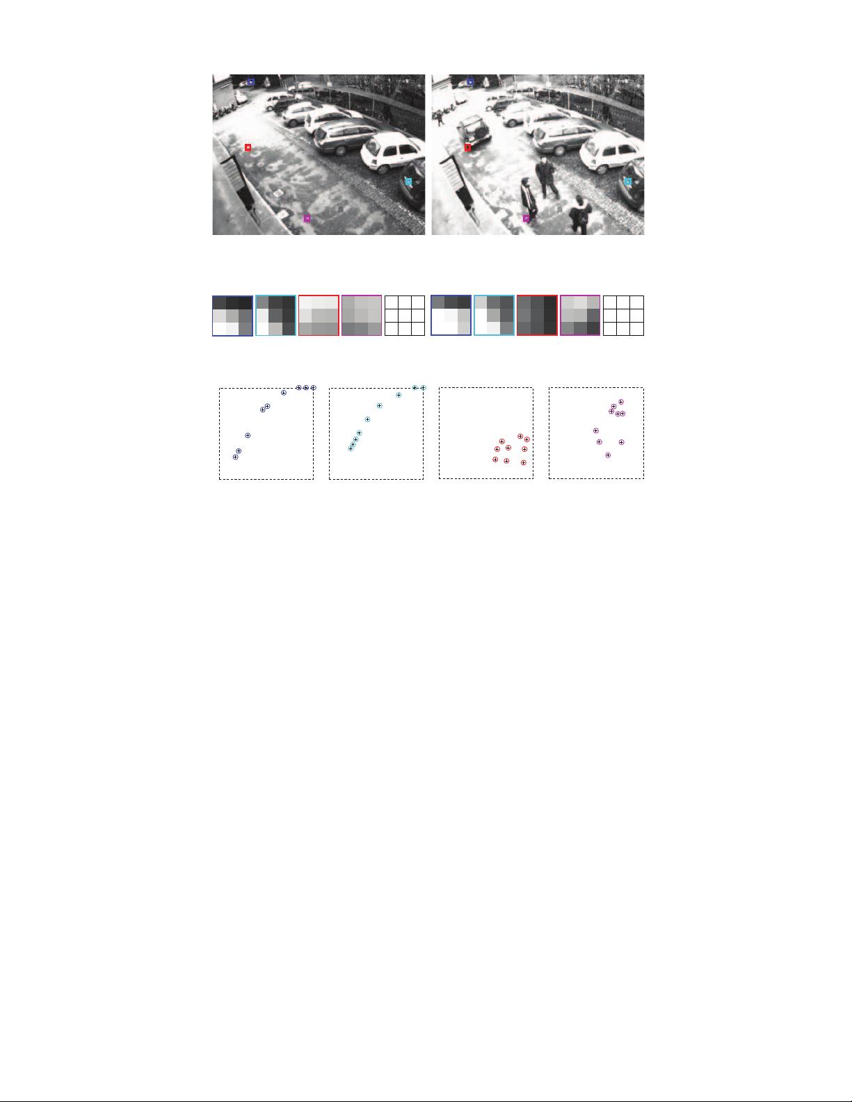
four sample 3 × 3 neighborhoods in the background (left) and in the current frame (right)
corresponding, respectively, to two unchanged (blue and azure border) and two changed (red and
violet border) pixels
[
[
[
[
[
[
[
[
[
\
\
\
\
\
\
\
\
\
(b)
enlarged background (left) and current frame (right) neighborhoods with adopted notations
for sensed pixel intensities
[
\
[
\
[
\
[
\
(c)
feature vectors representation in the (x, y) cartesian plane for the two unchanged (left) and
the two changed (right) pixels
Fig. 1. Representation of the feature vector f =(x
1
,...,x
N
,y
1
,...,y
N
) in the (x, y) plane (c) for four 3 × 3 square neighborhoods (a,b) in a sample
frame of an outdoor video sequence sensing strong photometric changes with respect to the background. The neighborhoods correspond, respectively, to two
unchanged (blue, azure) and two changed (red, violet) pixels.
made about foreground objects appearance (e.g. color and
shape) or, as for the priors, information other than f is
exploited, scene changes do not yield statistically predictable
patterns neither in our simple intensity feature space nor in any
other neighborhood-based feature space. Examples of different
image change patterns are shown in Fig. 1(c), with the two
leftmost scatter plots depicting predictable patterns yielded
by disturbance factors and the two rightmost showing unpre-
dictable patterns due to the presence of foreground objects.
As a consequence, only information related to class U can be
exploited for change detection. In particular, scene changes
can only be detected by a-contrario testing the hypothesis that
observed feature vectors are due to disturbance factors, so that
change detection reduces to a statistical test formalizable, in
general, as follows:
C
t(U, f) ≷ T
U
(7)
where t(U, f ) is a test statistic providing a statistical measure
of the distance between the two events, respectively, of only
disturbance factors acting in the considered patch and of
feature vector f being sensed, T is the test threshold allowing
for tuning the desired sensitivity vs specificity tradeoff. Hence,
change detection requires statistical modeling of, and only of,
information related to class U . In other words, the possible
effects of disturbance factors on a neighborhood of pixel
intensities have to be modeled in order to make the test in (7)
explicit.
IV. M
ODELING OF DISTURBANCE FACTORS EFFECTS
We assume main disturbance factors yielding changes of
pixel intensities over time to be imaging process noise, adjust-
ments of camera parameters (e.g. auto-exposure, auto-gain),
illumination changes. We do not consider the moving back-
ground problem (e.g. waving trees), for which the methods
belonging to the first category mentioned in Section I are more
suitable. Coherently with the notations in (2),(3) let us denote
the ideal noiseless feature vector as
˜
f =(
˜
x
˜
y)= (˜x
1
,...,˜x
N
, ˜y
1
,...,˜y
N
) ∈
F (8)
where
F =[0,L− 1]
2N
⊂ R
2N
(9)
is the (continuous) noiseless feature space. As in [11] and [16],
we model the imaging process noise as an additive, zero-mean,
independent gaussian disturb, so that the probability of observ-
ing the noisy feature vector f given its noiseless counterpart
˜
f is a 2N -variate gaussian
p(f |
˜
f)=N
f |
˜
f, Σ
f
(10)
with mean equal to the noiseless feature vector
˜
f and diagonal
covariance matrix
Σ
f
= diag
σ
2
(x
1
),...,σ
2
(x
N
),σ
2
(y
1
)),...,σ
2
(y
N
)
(11)
IEEE TRANSACTIONS ON PATTERN ANALYSIS AND MACHINE INTELLIGENCE
This article has been accepted for publication in a future issue of this journal, but has not been fully edited. Content may change prior to final publication.


