梯度引导边缘增强的多模态脑MRI超分辨率图像重建

31 浏览量更新于2024-08-31 收藏 1.33MB PDF 举报

本文档探讨了一项名为"Multi-Contrast Brain MRI Image Super-Resolution with Gradient-Guided Edge Enhancement"的研究，发表于2018年8月1日接收，9月21日接受，并在同年10月2日正式发布，最新版本日期为10月29日。该研究关注的是多模态脑磁共振成像(MRI)图像的超分辨率重建技术，特别强调了利用梯度引导边缘增强的方法来提升图像质量和细节。 MRI图像的高分辨率重建对于神经科学研究、临床诊断和治疗至关重要。传统MRI由于受到物理限制，如采样不足，可能导致图像模糊，难以捕捉到微小的结构变化。通过多对比成像，可以获取不同层面的信息，但处理这些复杂数据并提高空间分辨率是一项挑战。这项研究提出了一种创新的方法，即结合多模态MRI的不同对比度信息，并利用梯度信息指导边缘增强，以增强图像的边缘清晰度，从而实现超分辨率重建。在方法论上，研究者可能采用了先进的图像处理算法，例如深度学习或者基于稀疏表示的模型，将低分辨率图像与不同对比度的MRI序列融合。梯度引导部分可能涉及到对图像的局部梯度信息进行分析，以便确定哪些区域的边缘应该被强化，这有助于突出重要的解剖结构或病变特征。文章的关键贡献可能包括： 1. **高效算法设计**：开发了一种能有效整合多模态MRI数据的算法，同时考虑到梯度信息的指导，以优化图像质量。 2. **边缘增强策略**：提出了一种新的边缘增强策略，可能通过提升边缘细节，使医生能够更准确地识别和分析大脑结构。 3. **实际应用价值**：研究可能展示了在实际应用中的性能提升，比如在早期疾病检测、手术导航或疗效评估中的改进效果。此外，该研究可能还包含实验结果和对比分析，以验证新方法相对于传统方法在图像质量和重建速度上的优势，以及对临床应用的可行性进行了讨论。这篇研究论文是IT领域的一个重要贡献，特别是在医疗成像技术的发展方向上，为多模态脑MRI图像的解析提供了创新的解决方案，具有显著的实际应用前景。

H. Zheng et al.: Multi-Contrast Brain MRI Image Super-Resolution With Gradient-Guided Edge Enhancement

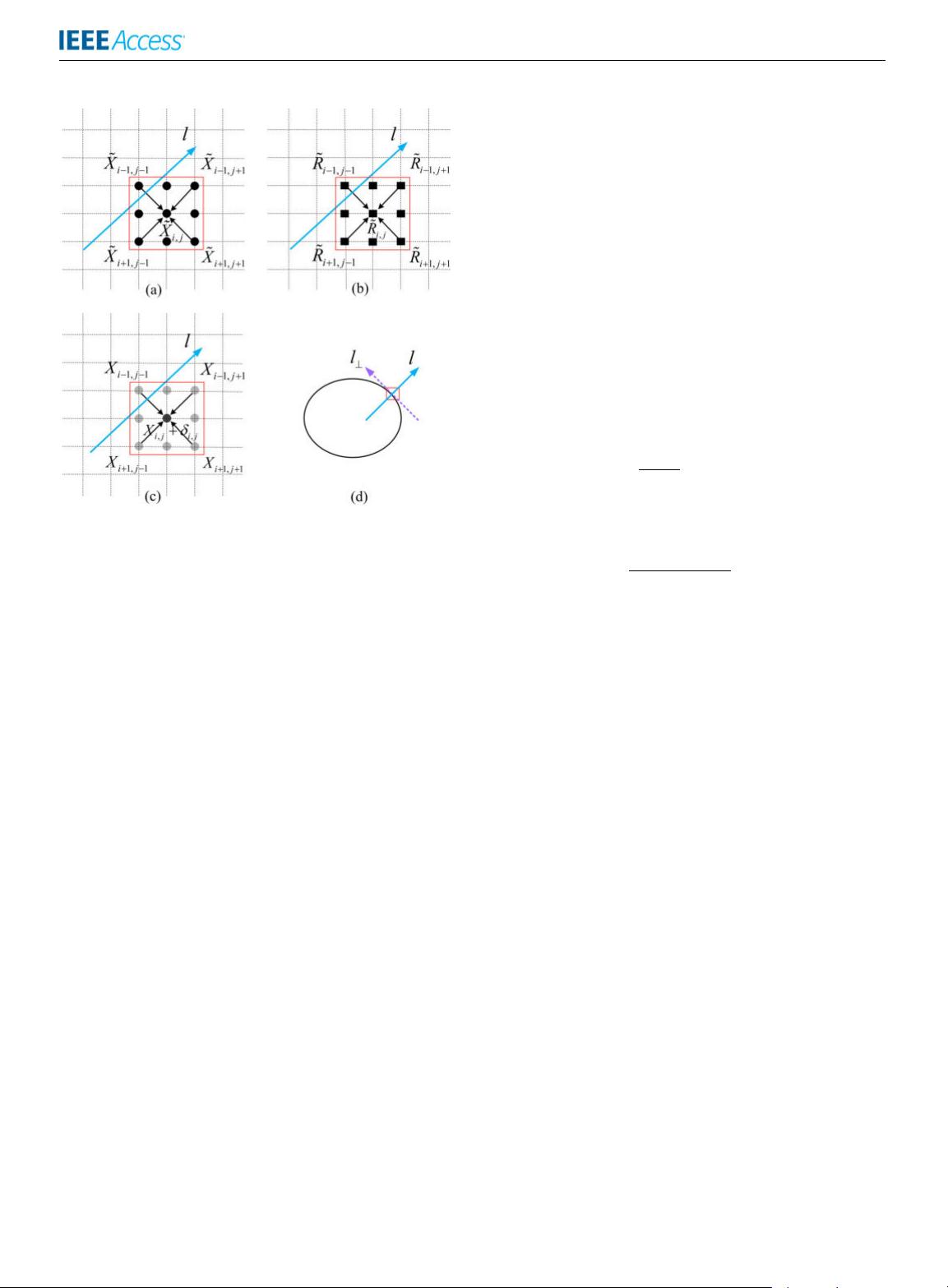
FIGURE 2. Illustration for SRGR model in a local pattern. (a) is the target

HR image

X; (b) is the HR reference image

R with different contrast; (c) is

the pre-interpolated image X obtained from the low observation of

(d) An example of the gradient direction l in a local pattern and the edge

direction. Note: The gradient direction is denoted by the vector l.

In estimation, a more accurate pixel, e.g. X

i,j

+ δ

i,j

, indicated by dark

circles within (c) is used to replace the pre-interpolated HR pixel,

e.g. X

i,j

, to generate a better HR image.

where X

i+1,j−1

and X

i−1,j+1

are the neighborhood pixels of

i,j

along the direction l, while X

i−1,j−1

and X

i+1,j+1

are the

nearest neighbors of X

i,j

along the direction l

⊥

, respectively.

Second, the λ and λ

⊥

in Eq. (

3) are parameters that adjusting

intensity in two directions. Too smaller λ and λ

⊥

will lead to

blur edges. On the contrary, too larger λ and λ

⊥

will cause

artiﬁcial edges [19]. In SRGR, their values are estimated as

λ = (X

i+1,j−1

− X

i−1,j+1

)/(

i+1,j−1

−

i−1,j+1

)

⊥

= (X

i−1,j−1

− X

i+1,j+1

)/(

i−1,j−1

−

i+1,j+1

). (5)

Overall, the SRGR model in Eq. (

3) tries to reﬁne the pixels

of pre-interpolated image by minimizing the consistent sec-

ond order gradient that is parallel and perpendicular to the

edges. Since each term in this model is quadratic, Eq. (

3) can

be solved fast by forcing the ﬁrst derivative of the objective

function to be zero. More details of implementation can be

found in [19].

However, the basic SRGR may not suit well for recovering

MRI since the local-contrast may be more complex than the

remote sensing images presented in [19]. How to modify the

SRGR to ﬁt for multi-contrast MRI will be the main focus of

our work.

III. PROPOSED METHOD

An overview of the proposed approach is summarized

in Fig. 3. First, the LR image is pre-interpolated by the

CGI method. Second, the HR reference image is registered

to pre-interpolated image (Beneﬁt of registration is shown in

Appendix C). Then, the HR image of interest will be restored

by using the gradient information of the registered HR ref-

erence image in another contrast. Finally, the HR image will

be enhanced with an IBP ﬁlter. In the following, the essential

parts of the proposed method will be presented.

A. MEASURING GRADIENT DIFFERENCE ON SAME

CONTRAST IMAGES

The essence of SRGR model in Eq. (3) is to estimate the

relationship of the second gradient order between the pre-

interpolated image X and the HR reference image

R. Now,

let us consider an ideal step. Assume that an ideal pre-

interpolation can generate a HR image X that is as good as

the target HR image

X. Accordingly, there may exist a pre-

interpolated reference image R that is as good as

R. Then,

according to Eq. (2), the following relationship holds true

g(X

i,j

)

g(R

i,j

)

≈ λ

, (6)

where R

i,j

is the (i, j) pixel of R. Through the elementary

mathematical manipulation of Eqs. (2) and (

6), one obtains

′

i,j

) − g(X

i,j

)

i,j

) − g(R

i,j

)

≈ λ

, (7)

which is the ratio of gradient difference estimated from the

same contrast images.

The Eq. (

7) implies that one may turn to measure the

ratio of the gradient difference for the pairs of target/pre-

interpolated images and reference/pre-interpolated reference

images. This modiﬁcation is important since the gradient

difference is computed within one contrast, but not across

two contrasts in the original SRGR in Eq. (2). Thus, Eq. (

is able to reduce the effect of large contrast variations on

degrading the multi-contrast MRI super-resolution, which

will be systematically analyzed in the following section.

B. SUPER-RESOLUTION MODEL

Based on Eq. (7), our model can be expressed as

min

i,j

{[(g(X

i,j

+ δ

i,j

) − g(X

i,j

)) − λ(g(

i,j

) − g(R

i,j

))]

+ [(g

⊥

i,j

+ δ

i,j

) − g

⊥

i,j

))

− λ

⊥

(

i,j

) − g

⊥

i,j

))]

} (8)

which ﬁnds reﬁnements on pixels to minimize the gradient

difference between the HR images and HR reference images.

In this model, the accuracy of λ and λ

⊥

is essential for

image reconstruction. Thus, error analysis on λ (same anal-

ysis for λ

⊥

is omitted) and edge pixels will be brieﬂy given

below (More details can be found in Appendix A). The fol-

lowing analysis will show that, comparing with the SRGR,

the new method will obtain lower reconstruction error on

edge pixels.

In our model, the error on λ is denoted by 1λ

′

deﬁned as

1λ

′

= λ

′

− λ, (9)

57858 VOLUME 6, 2018

剩余11页未读，继续阅读

weixin_38569109

粉丝: 7
资源: 955

梯度引导边缘增强的多模态脑MRI超分辨率图像重建

Image Super-Resolution using Gradient Profile Prior代码

Gradient Domain Guided Image Filtering

Structure-Preserving Super Resolution with Gradient Guidance

Modeling Deformable Gradient Compositions for Single-Image Super-resolution

Multi-focus image fusion using a binary gradient-based Sharpness criteria:Multifocus image fusion using a binary gradient-based Sharpness criteria-matlab开发

Edge-Preserving Image Smoothing with Local Constraints On Gradient And Intensity

Multi-band imaging and focusing of photonic crystal flat lens with scatterer-size gradient

Convergence of CR-gradient learning algorithm for Multi-valued Neuron

PyTorch-Image-Models-Multi-Label-Classification:基于timm的多标签分类

梯度域引导图滤波Gradient Domain Guided Image Filtering

最新资源