3
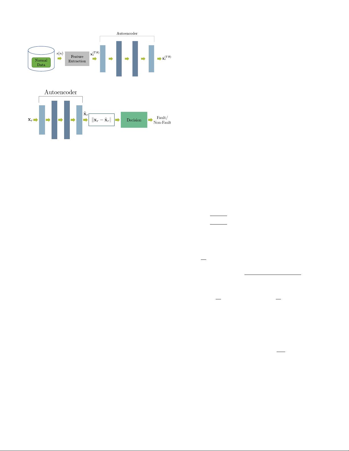
(a) Training phase.
(b) Fault detection phase.
Fig. 1. Block scheme of the proposed approach. In the training phase (a),
the superscript (T R) distinguishes a feature vector of the training phase from
the one of the test phase shown in (b).
from the measured vibration signals. The three architectures
have been evaluated by using a dataset created by the authors
and compared to the OC-SVM [33]. The results show that
the proposed neural networks-based algorithm outperforms the
OC-SVM approach, and that the MLP autoencoder provides
the overall highest performance.
III. PROPOSED METHOD
The block scheme of the proposed method is shown in
Fig. 1. Both in the training and in the detection phase, the
input signal is processed by the feature extraction stage,
where Log-Mel coefficients are calculated. Log-Mels are then
processed by a deep autoencoder, a neural network that is
trained to reconstruct its input [34]. During the training phase,
the autoencoder is trained by using only normal data, i.e.,
sequences that do not contain faults (Fig. 1a). In the detection
phase, the autoencoder takes as input the features extracted in
the feature extraction stage, but this time the signal can contain
a fault or not. In the first case, the reconstruction error is
expected to assume considerably higher values than the second
case. The “Decision” stage marks the input as a “Fault” if the
reconstruction error exceeds a certain threshold, otherwise as
“Non-Fault”. The remainder of this section describes in detail
the stages of the algorithm.
A. Feature extraction
The feature extraction stage reduces the dimensionality of
the input data, while retaining significant characteristics that
allow to discriminate whether an input sequence contains a
fault or not. In this paper, we used Log-Mel coefficients, a
set of spectral features that have been widely used for speech
applications [35], [36], but that have also been successfully
applied to the analysis of vibration signals [37], [38].
The first step for extracting Log-Mel coefficients is dividing
the input signal in frames of length 600 ms and overlapped by
300 ms (i.e., 50%). Overlapping two consecutive frames by
50% results in a good compromise between time-resolution
and computational requirements of the algorithm.
Denoting with s(n) the input signal and with w(n) the
window function, the r-th frame s
r
(m) of s(n) is defined
as:
s
r
(m) = s(rR + m)w(m), −∞ < r < ∞, 0 ≤ m ≤ L − 1,
(1)
where R is the frame step and L is the length of the window
w(n). A common choice for the window function is the
Hamming window, whose form is the following [39]:
w(n) =
0.54 − 0.46 cos (2πn/L) , 0 ≤ n ≤ L − 1,
0, otherwise.
(2)
The second step from extracting Log-Mels is calculating the
N-points Discrete Fourier Transform of s
r
(m):
S
r
(k) =
L−1
X
m=0
s
r
(m)e
−j(2π/N)km
, (3)
where k denotes the frequency bin.
Log-Mel coefficients are obtained by filtering S
r
(k) with
a filterbank composed of B triangular filters equally spaced
along the mel-scale, and then calculating the logarithm of the
energy in each band. The b-th triangular filter h
b
(k) of the
filterbank is calculated as follows [40]:
h
b
(k) =
0, k < f
b−1
,
k−f
b−1
f
b
−f
b−1
, f
b−1
≤ k < f
b
,
f
b+1
−k
f
b+1
−f
b
, f
b
≤ k < f
b+1
,
0 k ≥ f
b+1
,
b = 1, 2, . . . , B,
(4)
where the boundary frequencies f
b
are obtained as:
f
b
=
N
f
s
Mel
−1
(Mel(f
low
)+
+b ·
Mel(f
high
) − Mel(f
low
)
B + 1
, (5)
with
f
0
=
N
f
s
f
low
, f
B+1
=
N
f
s
f
high
, (6)
f
s
is the sampling frequency, and f
low
and f
high
are respec-
tively the lowest and highest frequencies of the filterbank. The
transformation Mel(·) and its inverse Mel
−1
(·) respectively
map a linear frequency into the mel scale and vice-versa, and
they are defined as follows [41]:
Mel(f) = 2595 log
10
1 +
f
700
, (7)
Mel
−1
(f) = 700
h
10
(f/2595)−1
i
. (8)
A single Log-Mel coefficient is then given by:
x
r
(b) = log
N−1
X
k=0
h
b
(k)|S
r
(k)|
2
!
. (9)
Since the filterbank is composed of B filters, the final feature
vector is structured as follows:
x
r
= [x
r
(1), . . . , x
r
(B)]
T
. (10)


