基于判别性度量学习的高光谱图像异常检测方法

需积分: 9 162 浏览量更新于2024-09-07 收藏 2.16MB PDF 举报

本文主要探讨了一种基于区分性度量学习的异常检测方法，针对高光谱图像中的异常检测问题。传统的基于马氏距离的异常检测方法依赖于背景统计信息来构建检测指标，但存在两个主要挑战：首先，对背景数据的高斯分布假设可能并不适用，这可能导致检测性能下降；其次，常规背景协方差矩阵容易受到异常像素的污染，从而影响异常检测的准确性。该论文提出了一种新颖的策略，通过有效利用区分性信息来增强异常像素与背景像素之间的分离度，从而提高异常检测的鲁棒性。这种方法的关键步骤包括两部分：首先，引入流形特征，将像素划分为潜在的异常区域和潜在的背景区域，这一过程称为区分性信息学习。这种划分有助于区分那些在光谱上显著不同的异常目标。接着，作者采用一种度量学习方法，旨在学习一个更为稳健的异常程度度量，这个度量能够更准确地衡量每个像素属于异常类的概率，减少由背景噪声或异常样本对异常检测结果的影响。这种方法不仅考虑了全局背景统计，还结合了局部结构信息，提高了异常检测的准确性和稳定性。通过对三个不同高光谱数据集的实验验证，研究结果表明，这种基于区分性度量学习的异常检测方法在性能上优于现有的传统方法。它在异常检测的敏感性和精确性方面都表现出优势，尤其是在处理那些光谱特性显著不同于背景的数据时，其效果尤为显著。本文提供了一个有效的解决方案，通过结合流形特征和度量学习技术，有效地解决了高光谱图像异常检测中的背景假设问题和异常污染问题，对于提高遥感领域中的目标识别和异常事件检测具有重要意义。

6846 IEEE TRANSACTIONS ON GEOSCIENCE AND REMOTE SENSING, VOL. 52, NO. 11, NOVEMBER 2014

be imposed to be zero for those x

that are not among them;

second, the rows of the weight matrix should be summed to

be one. By the two constraints, the reconstruction errors are

invariant to rotations, rescalings, and translations of that data

pixel and its neighboring pixels. From (1), the invariance to

rotations and rescalings follows immediately; the invariance to

translations is enforced by the sum-to-one constraint on the

rows of the weight matrix. The optimal ω

(i)

to the cost error

then becomes a constrained optimization problem. Detailed

information on the solution is included in Appendix I.

Suppose that the data set also lies on or near a smooth

nonlinear manifold of dimensionality d(d  L). There would

then be a proper linear mapping, which employs translation, ro-

tation, and rescaling, to map the high-dimensional coordinates

of each neighborhood into the global internal coordinates on

the manifold [29]. These corresponding reconstruction weights

should directly reﬂect the intrinsic geometric properties of the

data set, so that it would not be variant to these transforma-

tions. In other words, each locally linear patch from the high-

dimensional feature space can be placed in a low-dimensional

embedding space, where the same weight ω

that reconstructs

the ith pixel in the L dimensions should also reconstruct its

embedded manifold coordinates in d dimensions.

The key to the low-dimensional embedding is then a neigh-

borhood preserving mapping. Therefore, each pixel x

mapped into a low-dimensional vector z

to minimize the

embedding cost function:

ε(z)=



i=1



−



∈H



. (3)

The aforementioned cost function is much like the previous

one, which is also computed from the locally linear reconstruc-

tion errors. The weight ω

is ﬁxed this time, and the embedding

cost in the aforementioned equation constitutes a minimization

problem. The solution actually becomes a sparse eigenvec-

tor problem. The ﬁnal z

constitutes the bottom d nonzero

eigenvectors, which constitute an ordered set of orthogonal

coordinates centered on the origin. Further details are listed in

Appendix II.

In the aforementioned way, each pixel’s reconstruction

weight is retrieved by only its local neighborhood pixels. In

other words, each patch is independent of the other patches

in the mapping into the low-dimensional feature space. By the

weight matrix, however, a global operation coupling all of the

pixels in the connected components of the graph of the matrix

is constructed, and an N

∗

N eigensolver is computed to get the

embedding coordinates. In addition, the bottom eigenvectors

from (3) are ﬁgured out one at a time. In this way, all of the local

patch information is exploited to discover the global structure,

as all of the pixels’ patches are overlapping.

We use the reconstruction error in (3) as the separation rule,

with adaptive thresholding [2], which is quick and increases the

ﬂexibility, so as not to omit the probable anomalies. Further-

more, the anomalies have a low probability of occurrence in the

image, and the percentage of target pixels versus background

is under 1%. In most cases, we can safely use an empirical

probability of 0.05% for separating the most probable anomaly

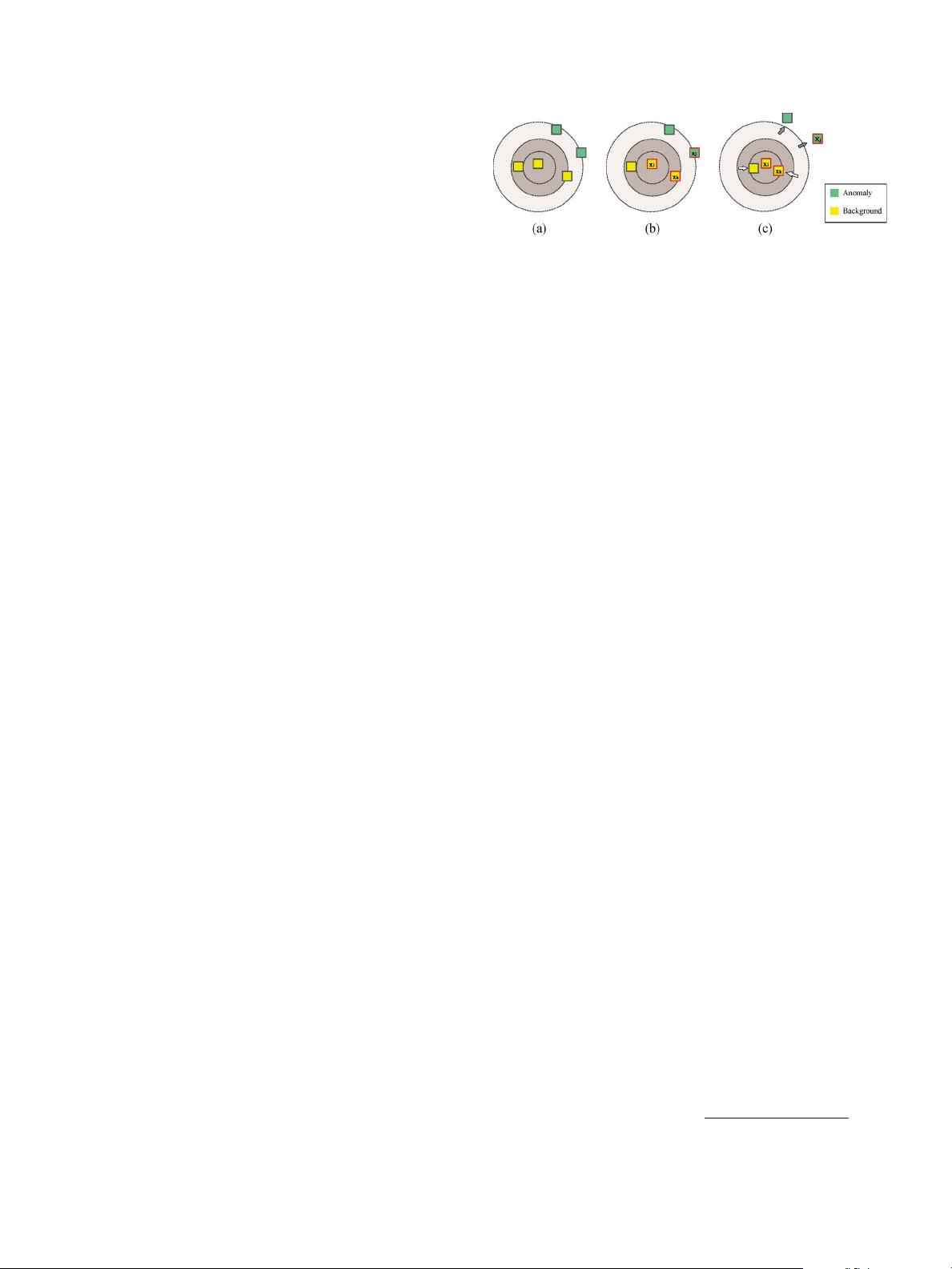
Fig. 2. Schematic illustration of the proposed method. The purpose is to

enlarge the separability between anomalies and background pixels, while the

distance of background pixels is reduced. (A) Original sample. (B) Triplewise

discriminative information labeling. (C) Projecting by anomaly metric.

pixels. The adaptive thresholding method then calculates the

threshold for segmenting anomalies by setting an accumulat-

ing distribution probability percentage of 99.95% from the

histogram of the detection results. The determined probable

anomaly areas are not used directly as the detection results but

as the discriminative label information.

We deﬁne two sets named A (anomaly) and B (background)

to denote these labels. For each anomaly pixel, two of its

surrounding nearest neighbor background pixels are picked up

to construct the two data sets. The two background pixels refer

to those among the observed anomaly pixel’s neighbors but are

also the ones with low reconstruction errors to be classiﬁed

as background pixels. Therefore, the number of B is twice

of that of A(N

=2N

). We can then deﬁne the dissimilar

data set D and the similar data set S from these two sets:

D = {(x

, x

)}, x

, x

=1,...,N

, where x

belongs to B

and x

belongs to A, with x

being the nearest neighbor of

in B; S = {(x

, x

)}, x

, x

=1,...,N

, where x

and

belong to B. Furthermore, a guard interval is set between

the labeled anomaly pixels and the labeled background pixels,

excluding the labeled background pixels with the largest 10%

reconstruction errors, so as to make S and D immune to weak

anomalies on the boundary of anomaly and background.

III. A

NOMALY METRIC LEARNING

AND

ANOMALY DETECTION

The main idea behind our method can be represented as

follows. From Fig. 2(a), the anomaly pixels appear to be not

particularly differentiable from the background ones. Then, in

Fig. 2(b), the pixels are labeled as probable anomaly and prob-

able background by means of the manifold reconstruction error.

Finally, with the aim of improving the separability between

anomalies and backgrounds, all of the samples are projected

by a proper anomaly metric. The resulting distribution is shown

in Fig. 2(c), revealing that the background samples are more

compact, while the distances between the backgrounds and

anomalies are enlarged.

The key then becomes the construction of a robust anomaly

metric from the label information. A Mahalanobis-like distance

metric is employed. Its expression is

dis

, x

)=x

−x





−x

)

M(x

−x

). (4)

In order to ﬁgure out M, an optimal function should be

deﬁned. Some distance constraints are also introduced. In de-

tail, the optimal function comprises two parts: The ﬁrst part

剩余13页未读，继续阅读

mning_master0

粉丝: 1
资源: 18

基于判别性度量学习的高光谱图像异常检测方法

Enhancing the Discriminative Feature Learning for Visible-Thermal Cross-Modality

Locality Sensitive Discriminative Dictionary Learning

deepcnn人脸识别center loss（discriminative feature learning）

salient object detection: a discriminative approach

DIscriminative-Learning-in-Semantic-Segmentation-on-Cityscape-Dataset:使用Pytorch的判别学习使用Pretrained Resnet 18模型训练Cityscape数据

Discriminative Analysis Dictionary Learning

ROBUST OBJECT TRACKING VIA ONLINE MULTIPLE INSTANCE METRIC LEARNING

Discriminative Learning of Local Image Descriptors

Matlab code for Learning a discriminative high-fidelity dictionary for SCSS

[CVPR 2018]Discriminative Learning of Latent Features for Zero-Shot Recognition

最新资源