深度学习详解：Transformer与GNN的最新进展

下载需积分: 25 | PDF格式 | 5.37MB | 更新于2024-06-29 | 38 浏览量 | 举报

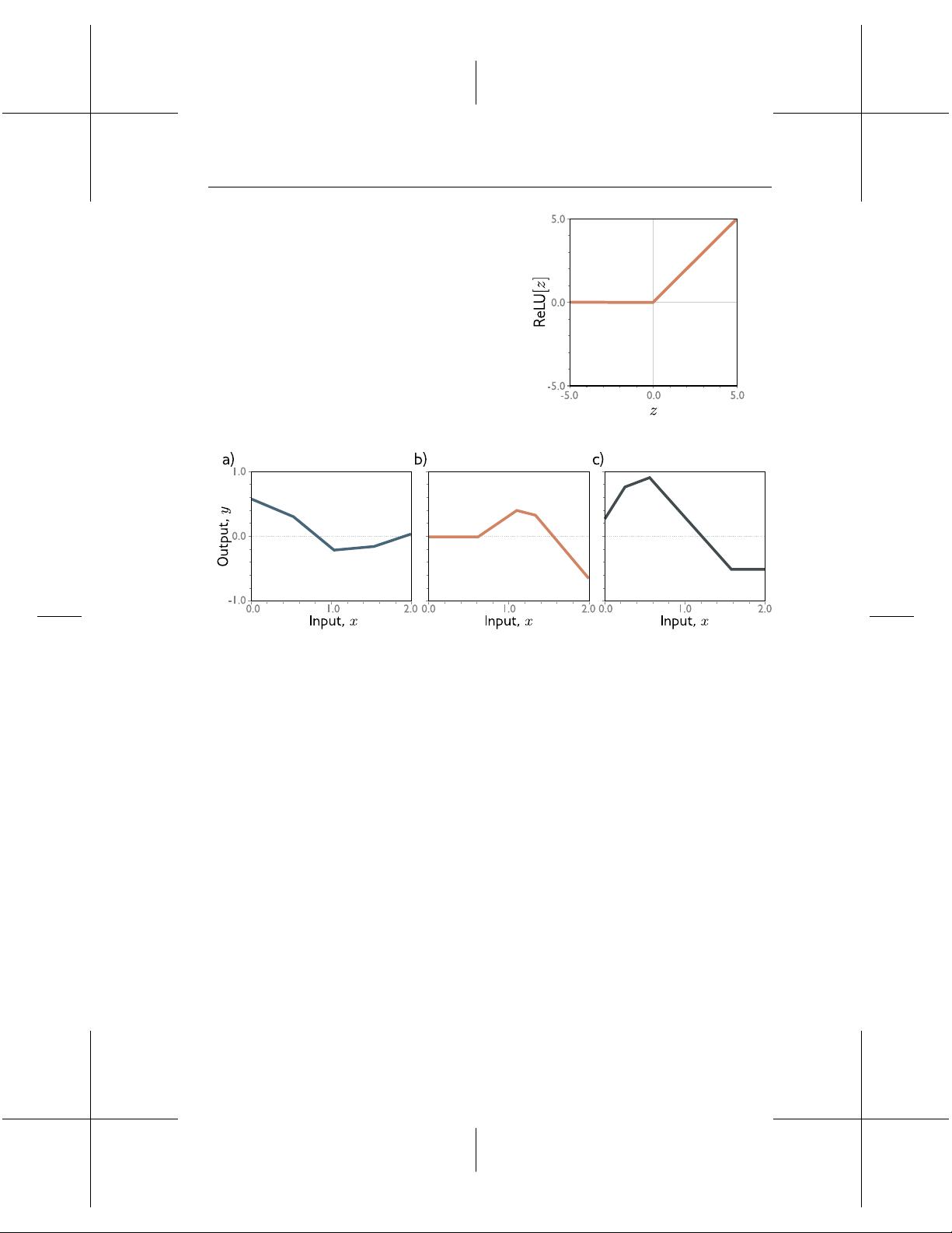
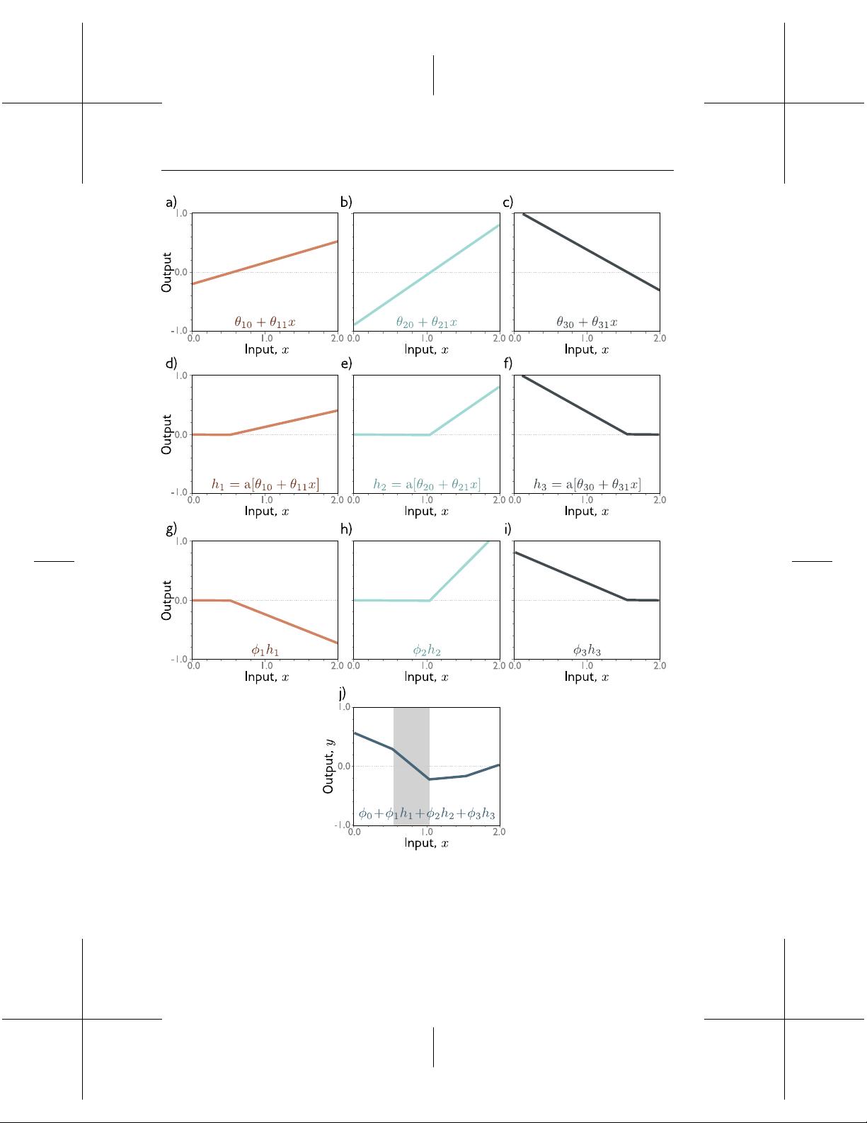
深度学习是现代人工智能的核心组成部分，它是一种模仿人脑神经网络结构和功能的计算模型，用于处理复杂的数据模式和高级任务。在本资源中，作者Simon J. Prince带领读者逐步理解深度学习的基本概念和最新进展，特别关注了Transformer和图神经网络（GNN）这两种前沿技术。第1章"Introduction"介绍了深度学习的背景和重要性，强调了其在机器学习领域的核心地位，以及与传统统计方法的区别。章节通过实际案例，如线性回归，展示了监督学习的基础，包括模型的构建、损失函数的选择和训练过程，以帮助读者建立对基本概念的理解。接着，第2章深入探讨了浅层神经网络，这部分内容包括神经网络的工作原理，如神经元之间的连接和权重更新。"Universal approximation theorem"指出神经网络具有强大的表达能力，可以近似任何连续函数，这对于理解深度学习的潜力至关重要。同时，该章节也讨论了多变量输入和输出的情况，通过可视化工具来帮助读者直观感受数据的维度变化。进入21世纪的最新进展，第3章重点讲解了Transformer模型。Transformer是基于自注意力机制的架构，最初在自然语言处理中的大规模预训练模型如BERT和GPT系列中取得了显著成功。它摒弃了传统的循环或卷积结构，能够并行处理序列数据，极大地提高了模型的效率和性能。这一部分会深入解析Transformer的工作原理，并与传统神经网络进行对比。此外，图神经网络（GNN）在第4章被详细阐述，这是针对网络数据（如社交网络、分子结构等）设计的一种特殊类型的深度学习模型。GNN通过聚合邻居节点的信息，学习图结构中的局部特征表示，这在推荐系统、社区检测和药物发现等领域有广泛应用。整个资源旨在提供一个全面且易于理解的深度学习入门指南，涵盖了基础知识、实践技巧和前沿技术，帮助读者在不断发展的AI领域中跟上步伐。同时，作者鼓励读者积极参与反馈，共同提升文档质量。无论是对初学者还是专业人士，这份资源都是一份宝贵的参考资料。

展开

14 2 Supervised learning

terms on the right-hand side of equation 2.5) and the cost function is the overall quantity

that is minimized (

i.e.

, the entire right-hand side of equation 2.5). A cost function

can contain additional terms that are not associated with individual data points. More

generally, an objective function is any function that is to be maximized or minimized.

Generative vs. discriminative models: The models y = f[x, ϕ] in this chapter are

discriminative models. These make an output prediction y from real-world measurements

x. Another approach is to build a generative model x = g[y, ϕ], in which the real-world

Problem 2.3

measurements x are computed as a function of the output y.

The generative approach has the disadvantage that it doesn’t directly predict y. To

perform inference, we must invert the generative equation as y = g

−1

[x, ϕ] and this may

be dicult. However, generative models have the advantage that we can build in prior

knowledge about how the data were generated. For example, if we wanted to predict the

3D position and orientation y of a car in an image x, then we could build knowledge

about car shape, 3D geometry, and light transport into the function x = g[y, ϕ].

This seems like a good idea, but in fact, discriminative models dominate modern machine

learning; any advantage gained from exploiting prior knowledge in generative models is

usually trumped by brute force learning of very exible discriminative models from large

amounts of training data.

Problems

Problem 2.1 To walk ‘downhill’ on the loss function (equation 2.5), we measure its slope

with respect to the parameters ϕ

and ϕ

. Calculate expressions for the slopes ∂L/∂ϕ

and ∂L/∂ϕ

Problem 2.2 Show that we can nd the minimum of the loss function in closed form by

setting the expression for the derivatives from problem 2.1 to zero and solving for ϕ

and

. Note that this works for linear regression but not for more complex models; this is

why we use iterative model tting methods like gradient descent (gure 2.4).

Problem 2.3 Consider reformulating linear regression as a generative model so we have

x = g[y, ϕ] = ϕ

+ ϕ

y. What is the new loss function? Find an expression for the inverse

function y = g

−1

[x, ϕ] that we would use to perform inference. Will this model make the

same predictions as the discriminative version for a given training dataset {x

, y

This work is subject to a Creative Commons CC-BY-NC-ND license. (C) MIT Press.

18 3 Shallow neural networks

= a[θ

+ θ

= a[θ

+ θ

= a[θ

+ θ

x], (3.3)

where we refer to h

, h

, and h

as hidden units. Second, we compute the output

by combining these hidden units with a linear function:

y = ϕ

+ ϕ

. (3.4)

Figure 3.3 shows the ow of computation that creates the function in gure 3.2a.

Each hidden unit contains a linear function θ

•0

+ θ

•0

x of the input, and that line is

clipped by the ReLU function a[•] below zero. The positions where the three lines

cross zero become the three “joints” in the nal output. The three clipped lines

are then weighted by ϕ

, ϕ

, and ϕ

respectively. Finally, the oset ϕ

is added,

which controls the overall height of the nal function.

Problems 3.2-3.8

Each linear region in gure 3.3j corresponds to a dierent activation pattern

in the hidden units. When a unit is clipped, we refer to it as inactive, and when

it is not clipped, we refer to it as active. For example, the shaded region receives

contributions from h

and h

(which are active) but not from h

(which is inactive).

The slope of each linear region is determined by (i) the original slopes θ

•1

of the

active inputs for this region, and (ii) the weights ϕ

•

that were subsequently applied.

For example, the slope in the shaded region is θ

+ θ

Each hidden unit contributes one ‘joint’ to the function, so with three hidden

units, there can be four linear regions. However, only three of the slopes of these

regions are independent; the fourth is either zero (if all the hidden units are inactive

Problem 3.9

in this region) or is a sum of slopes from the other regions.

3.1.2 Depicting neural networks

We have been discussing a neural network with one input, one output, and three

hidden units. We visualize this network in gure 3.4a. The input is on the left,

the hidden units are in the middle, and the output is on the right. Viewed in

this way, each connection represents one of the ten parameters. To simplify this

representation, we do not typically draw the intercept parameters, and so this

network would usually be depicted as in gure 3.4b.

A linear function has the form z

′

= ϕ

∑

. Any other type of function is non-linear.

For instance, the ReLU function (equation 3.2) and the example neural network that contains it

(equation 3.1) are both non-linear.

This work is subject to a Creative Commons CC-BY-NC-ND license. (C) MIT Press.

剩余202页未读，继续阅读

身份认证购VIP最低享 7 折!

30元优惠券

KerryMo

粉丝: 211

深度学习详解：Transformer与GNN的最新进展

Graph-Transformer:用于图形分类的变压器（Pytorch和Tensorflow）

精品--精选了千余项目，包括机器学习、深度学习、NLP、GNN、推荐系统、生物医药、机器视觉、前后端开发等内容。.zip

gnn加transformer模型，扣除背景

GNN/GCN与Transformer结合的多模态对话情感识别项目

NLP实践demo，包含了文本分类，对话机器人，Transformer, GPT实现，图神经网络GNN使用，对抗训练，摘要抽取等

视觉Transformer

深度学习模型，相关学习的网络

深度学习革命性突破：1000层Transformer模型问世

利用谱注意力革新图Transformer：从光谱角度理解位置编码

深度学习模型集成大比拼：Transformer-Unet与其它模型的性能对决

最新资源