分布式轨道占用检测方法

81 浏览量更新于2024-08-28 收藏 1.12MB PDF 举报

"分布式轨道占用检测方法" 这篇论文探讨了在分布式环境下的轨道占用检测问题。轨道占用检测是铁路系统中确定哪条轨道被占用的关键任务。对于每条轨道，研究者应用了Neyman-Pearson检验框架来做出局部决策。从全局角度来看，这是一个多假设测试问题。文中采用了贝叶斯方法来最小化全球决策错误的概率。基于多个假设的先验概率和局部接收操作特性曲线的近似值，该方法旨在优化决策效率。 Neyman-Pearson检验是一种经典的统计决策理论，用于在给定假定的错误类型（第一类错误和第二类错误）下，确定最佳的阈值来区分两个对立的假设。在这个应用中，每个轨道的占用状态被视为一个独立的假设，通过Neyman-Pearson准则进行分析，以最大程度地降低错误检测的可能性。分布式检测的概念则强调了在多传感器或分布式节点之间协同工作以完成检测任务的重要性。在铁路系统的背景下，这意味着各个监测点可以独立地分析其覆盖范围内的轨道状态，并将结果整合到一个全局的决策过程中。这样可以提高系统的可靠性和鲁棒性，因为即使某些局部节点故障，整个网络仍能继续运行。贝叶斯方法是一种统计推理技术，它利用先验信息（即在观察数据之前已知的信息）来更新对事件发生概率的估计。在轨道占用检测中，先验概率可能包括历史数据、轨道的预期使用模式或者特定时间的交通流量等信息。通过结合先验和观测数据，贝叶斯方法可以生成后验概率，从而帮助做出更准确的占用状态判断。此外，通用似然比测试（Generalized Likelihood Ratio Test, GLRT）在多假设测试中也发挥了作用。GLRT提供了一种评估不同假设下数据似然性的方法，通常用于确定哪个假设最能解释观察到的数据。在轨道占用检测问题中，GLRT可能被用来比较不同轨道占用情况的似然性，以确定最有可能的情况。这篇论文提出了一种结合了Neyman-Pearson检验、贝叶斯方法和分布式检测策略的综合解决方案，旨在提升铁路系统的轨道占用检测性能。这种方法不仅考虑了局部决策的准确性，还考虑了全局决策的风险，从而提高了整体的决策效率和系统性能。

combining the Neyman–Pearson structure and the Bayesia n appro-

ach is formulated.

The rest of this paper is organized as follows. Section 2 describes

the local detection problem and its solutions. The distributed frame-

work and its fusion rule are presented in Section 3. As an illustration

of practical applications, a distributed track occupancy detection

problem in a group with three segments is provided in Section 4.

Some performance comparisons between the global decision with

and without the dynamical thresholds and the fusion rule are also

discussed here. Conclusions are summarized in Section 5.

2. Local detection

Track occupancy detection is achieved by a set of track circuits.

For each track circuit, there is a transmitter and a receiver

equipped on both ends. An approximate sinusoidal signal is

propagated from the transmitter to the receiver continuously

along the track. A track segment can be regarded as a concatena-

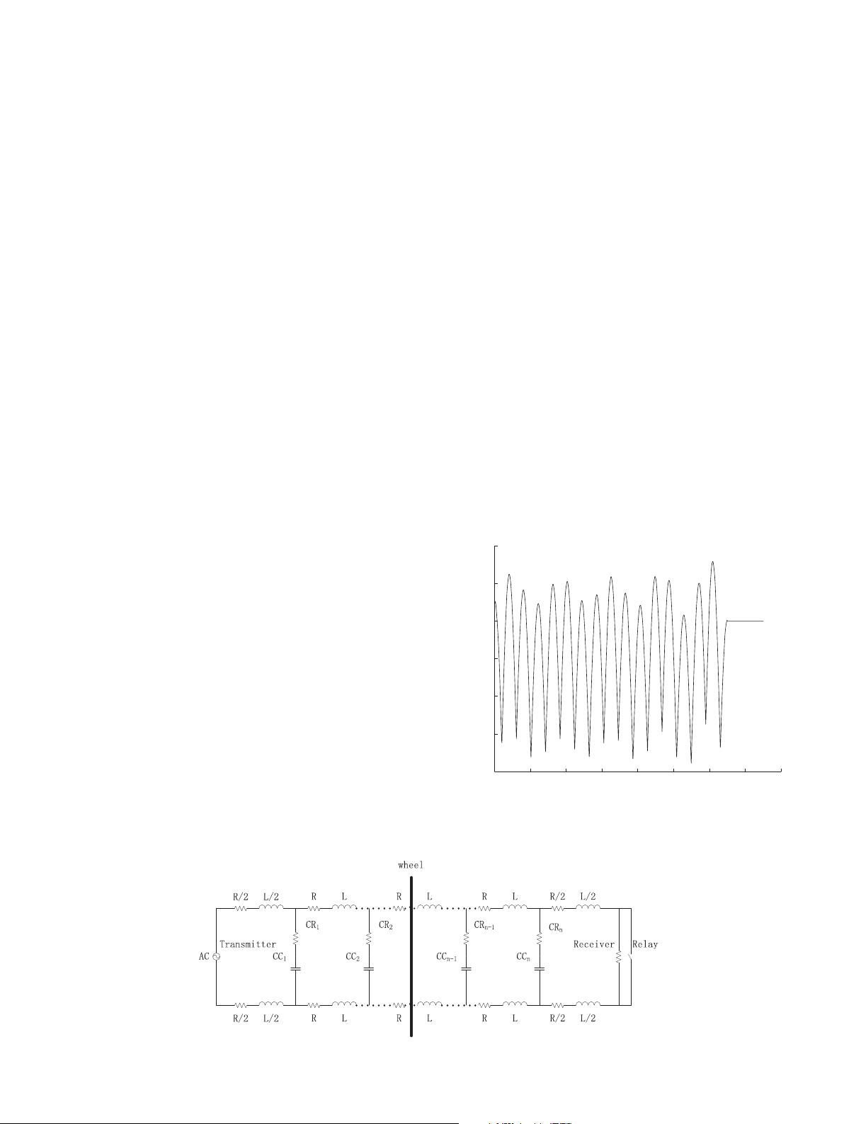
tion of resistances R and inductances L (Zhao et al., 2009). Along

the track, several complementary capacitors CC are ﬁxed, equally

spaced to neutralize the effect of inductances L. For each CC, there

exists a contact resistance CR linked to the track. The circuit

diagram of each track circuit is shown in Fig. 1 .

When there is a train on the track, signal propagation is shunted

by the front wheels of the train. Consequently, the receiving signal

decreases greatly. A relay is installed in the receiver to capture the

amplitude. If the receiving signal drops below a threshold, the relay

is triggered to activate a light corresponding to the current track on

the panel.

The curve of the receiving signal when the track is occupied can

be computed according to Zhao et al. (2009) and Zhao, Wu, and

Ran (2012). It is determined by the train position x on the track.

The receiving signal is denoted as U(x). Consider a typical track

circuit equipped with 16 complementary capacitors. When a train

passes through, the receiving signal is delineated in Fig. 2. While, if

the track is empty, the amplitude is a constant value.

As shown in Fig. 2, when a train passes through the track, the

receiving signal appears to be a position-related signal. Suppose

that the velocity is constant, then the sequential measurements

should be in accordance with such a curve except for an additive

noise. If the track is empty, the sequential measurements are iid.

Those are determined by a constant level plus a Gaussian noise.

Hence, there are two different modes to be distinguished.

2.1. Local detection formulation

The local detection is considered as a binary hypothesis testing

problem. H

means that the track is empty and H

means that the

track is occupied. A sliding window is applied here. In the sliding

window, there is a data block. For any two consecutive data blocks,

there is no overlap. Then the detection problem for segment i and

data block K is formulated as follows:

: y

¼Aþw

¼x

k 1

þvΔt

¼Uðx

Þþw

(

k ¼ðK 1ÞN; ðK 1ÞN þ1; …; KN 1 ð1Þ

where



i ¼1; …; n is the index of segments;



K ¼1; 2; … is the index of data blocks;



N is the size of the sliding window;



is the measurement of the receiving signal at time k in

segment i;



A is the receiving signal when the track is empty;



N ð0; s

Þ is the iid Gaussian noise at time k in segment i;



is the position of the train head at time k in segment i;



v is the velocity of the train, supposed to be constant;



Δt is the sample time; and



Uðx

Þ is the receiving signal when the track is occupied.

Remark 1. Suppose that for each track, the direction is well deﬁned

and all the tracks are connected sequentially. For some special cases,

i.e., cross/branched sections, parallel/cyclic tracks, train route infor-

mation provided by the interlocking is used to sequence the tracks.

Then all the tracks, despite their topologies, are connected sequen-

tially in logical level.

Fig. 1. Circuit diagram of each track circuit.

0 200 400 600 800 1000 1200 1400 1600

0.09

0.095

0.1

0.105

0.11

0.115

0.12

Position on the track (m)

Amplitude of voltage on the receiver (V)

Fig. 2. When the track is empty, the receiving signal is a constant value 0.6149 V,

otherwise a position-related signal.

M. Chang et al. / Control Engineering Practice 22 (2014) 69–80 71

剩余11页未读，继续阅读

weixin_38516386

粉丝: 5
资源: 899

分布式轨道占用检测方法

A Distributed Approach for Bitrate Selection in HTTP Adaptive Streaming.

Bigtable：A Distributed Storage System for Structured Data

Bigtable: A Distributed Storage System for Structured Data中文翻译

引用Distributed adaptive coverage control algorithm for mobile sensor networks

multisensor data fusion for next genera-tion distributed intrusion detection

Resilient Distributed Dataset

Apache Mesos frameworks

Hadoop Distributed File System

TimeDistributed is not defined

mapreduce近三年参考文献

最新资源