非线性异构Wiener过程模型的剩余使用寿命预测

124 浏览量更新于2024-08-27 收藏 2.4MB PDF 举报

"这篇研究论文探讨了非线性异构Wiener过程模型在剩余使用寿命预测中的应用，特别是在具有自适应漂移的情况下。作者Zeyi Huang, Zhengguo Xu, Wenhai Wang和Youxian Sun提出了一种新的模型，旨在处理实际系统中常见的非线性退化轨迹，并考虑其不均匀性。他们利用状态空间方法来定义模型，并解决了由于自适应漂移引入导致的Kalman滤波方法更新退化漂移分布的困难。为此，他们开发了一种基于贝叶斯定理的在线过滤算法。同时，他们采用了期望最大化(EM)算法以及一种新颖的基于贝叶斯定理的平滑器来估计模型中的未知参数。此外，论文还研究了预测剩余使用寿命(RUL)的分布情况。" 这篇论文主要关注的是在设备或系统的可靠性评估和预测领域，特别是对于那些退化过程非线性且不均匀的系统。Wiener过程是随机过程理论中的一种基本模型，常用于描述连续时间的随机变化，如设备的退化过程。在实际应用中，设备的退化往往不是线性的，也不总是均匀的，因此，传统的线性模型可能无法准确地捕捉这些复杂行为。作者提出的非线性异构Wiener过程模型引入了自适应漂移的概念，这使得模型能够适应退化轨迹的变化。然而，自适应漂移的引入对传统的Kalman滤波方法提出了挑战，因为这种方法通常假设模型参数是固定的。为了解决这个问题，他们设计了一种在线过滤算法，该算法基于贝叶斯定理，能够在获取新数据时动态更新退化漂移的分布。此外，论文还利用期望最大化(EM)算法来估计模型的未知参数。EM算法是一种迭代方法，通过最大化似然函数来估计参数，尤其适用于存在隐变量的情况。在本研究中，EM算法被用来优化模型参数，以更好地拟合观察到的退化数据。另一个创新点是采用了一种基于贝叶斯定理的新平滑器，它能够结合过去和当前的信息，提供对未知参数更精确的后验估计。这种平滑器对于理解和预测系统的未来状态至关重要，特别是预测剩余使用寿命(RUL)。这篇论文提供了处理非线性、异构退化问题的新方法，对于设备健康管理、故障预测和维护策略的制定具有重要意义。它展示了如何结合统计模型和概率方法来应对复杂的退化模式，有助于提高系统的可靠性和效率。

HUANG et al.: REMAINING USEFUL LIFE PREDICTION 689

model and Si's model are linear. It leads to the fact that both of

their models cannot trace the dynamics of nonlinear degradation

trajectories well.

From the above review of the related work, it can be found

that, though there is some research focusing on nonlinear degra-

dation trajectories or degradation models adaptive to historical

degradation data for RUL prediction, separately, few works con-

centrate on both of them simultaneously. As stated before, an

adaptive drift helps to take historical degradation data into ac-

count, and a nonlinear structure can make predicted degradation

trajectories close to actual degradation trajectories. The combi-

nation of an adaptive drift and a nonlinear structure contributes

to promoting the accuracy of RUL prediction. Accordingly, we

make three major contributions in this paper. First, we propose

a novel nonlinear heterogeneous Wiener-process-based model

with an adaptive drift for RUL prediction, and utilize a state-

space-based method to characterize our model. Second, we de-

velop an on-line ﬁltering algorithm based on Bayes' theorem

to update the hidden degradation drift, and then apply the ex-

pectation-maximization (EM) algorithm, and a novel Bayes'-

theorem-based smoother to estimate the unknown parameters

once a new measurement becomes available. Last, we derive

an explicit analytical distribution for the predicted RUL incor-

porating the complete distribution of the estimated degradation

drift.

The rest of this paper is organized as follows. In Section II,

we formulate the problem. In Section III, we develop an on-line

ﬁltering algorithm to estimate the degradation drift, and apply

the EM algorithm to re-estimate the unknown parameters. In

Section IV, we derive an explicit analytical distribution for the

predicted RUL. In Section V, a simulation, and a case study are

used to demonstrate the effectiveness of our model, and com-

pare the performance of our model with that of Wang's model,

and Si's model. Section VI concludes this paper.

II. P

ROBLEM FORMULATION

To take the complete historical degradation data into consid-

eration, as well as maintain the nice properties of the WP model,

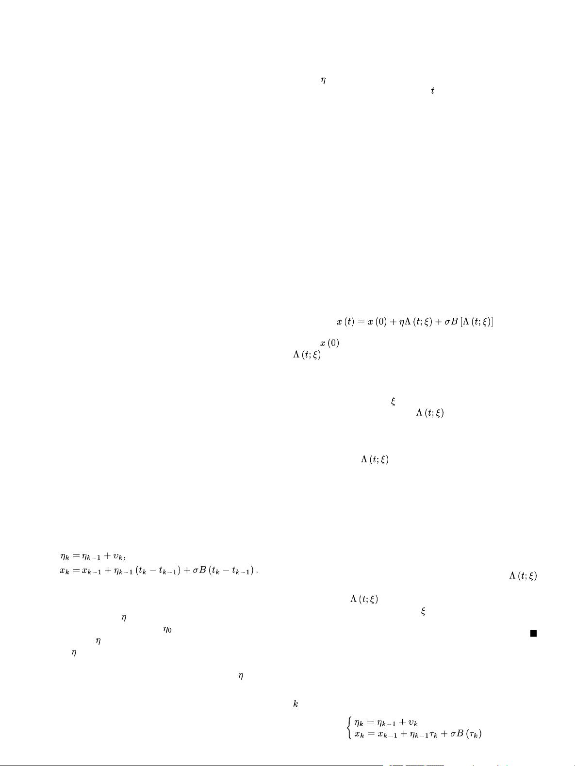
we consider Wang's model, given as [30]

(1)

(2)

In Wang's model, (2) was the discretized conventional WP

model, and the authors constructed an updating procedure for

the degradation drift

using a random walk model as in (1),

with the initial assumption that

followed a s-normal distri-

bution. Hence,

evolved as a time-dependent random variable.

Because

was unobservable, it had to be estimated once a new

measurement became available. Each time a new measurement

came out, they updated the posterior distribution of

using the

prior distribution and the new measurement by a recursive ﬁlter.

When the next measurement was available, the posterior distri-

bution at the current CM point became the prior distribution for

the next CM point. Thus, they established a link between the

historical degradation data and the predicted degradation levels

by incorporating the historical degradation data into the estima-

tion of

. Once the degradation drift was estimated, they used a

linear function with respect to time

to predict the evolution of

the degradation level.

However, in reality, nonlinear degradation trajectories are

encountered frequently, such as the degradation trajectories of

bearings [32], batteries [33], and gyros [34]. Thus, the linear

prediction used in the model described by (1) and (2) cannot

trace nonlinear degradation trajectories well. Additionally,

the conventional WP model is a time homogeneous process,

which means that the transition probability between two given

degradation states at any two CM points depends only on the

time interval. But not all degradation processes satisfy this

constraint. For example, the typical lifetime of the bearings

[35] can be roughly divided into two stages: one is the normal

stage, and the other is the defective stage. At the ﬁrst stage, the

bearings degrade slowly, whereas the defects propagate quickly

at the second stage. This example indicates that equally long

time intervals may give rise to different degradation increments.

To take nonlinearity and heterogeneity into consideration, we

incorporate a nonlinear structure into the WP model, given as

(3)

where

is usually assumed to be 0. The speciﬁc form of

can be determined by domain experts, or inferred from

the lifetime data of other identical systems. It is notable that

there are three advantages in (3). First, in contrast with the con-

ventional WP model, (3) can track nonlinear degradation trajec-

tories better by adjusting

to ﬁt the historical degradation data.

Second, the nonlinear function

can characterize a time

heterogeneous process. Third, as pointed out in [13], (3) retains

the nice mathematical property of the WP model that the explicit

distribution of the predicted RUL can be obtained analytically

once the form of

is speciﬁed.

Remark 1: There are two reasons for choosing a time-trans-

formation function instead of a more general one, e.g., a non-

linear drift used in [36], to characterize nonlinear degradation

trajectories. First, the explicit distribution of the predicted RUL

for the former can be obtained analytically, while the distribu-

tion of the predicted RUL for the latter is related to solving

the Fokker-Planck-Kolmogorov equation with boundary con-

straints, and the explicit analytical solution can be hardly ob-

tained. Second, members of a population of identical systems

have some common properties, so the speciﬁc form of

can be inferred from the lifetime data of other identical systems.

Subsequently,

can approach an individual degradation

trajectory through the adjustable

. Consequently, a time-trans-

formation function sufﬁces to characterize nonlinear degrada-

tion trajectories.

To better characterize practical degradation processes and ob-

tain the predicted RULs more accurately, we take nonlinearity,

heterogeneity, and the complete historical degradation data into

consideration simultaneously by combining (1) with (3). Ac-

cording to the Euler discretization, our complete model at the

th CM point is formulated as

(4)

剩余13页未读，继续阅读

weixin_38692969

粉丝: 4
资源: 953

非线性异构Wiener过程模型的剩余使用寿命预测

Remaining useful life prediction for a machine with multiple dependent features based on bayesian dynamic linear model and copulas

基于 Transformer 锂电池寿命预测（Remaining Useful Life，RUL）（Python完整源码和数据）

Adaptive Model Rules From High-Speed Data Streams

You have trained a TensorFlow model using Dropout layers for regularization. Now, youwant to use Monte Carlo Dropout for making predictions. What do you need to dodifferently during the prediction stage?

Adaptive Normalized Risk-Averting Training for Deep Neural Networks

Explain, with code snippets, how you have loaded your model to avoid incurring long waiting times for each classification.

prediction interval coverage probability

最新资源