
State
New'
block
Block-
chain
agent
Block'
template
PoUW
Miner
PoUW
Enclave
Blockchain'P2P'
Network'
TEE
Useful'
tasks
Useful'
results
State
Blockchain Agen t
Content
Compliance
Effort
Verifiers
1
2
2
3
4
5
6
Useful7
Work
client
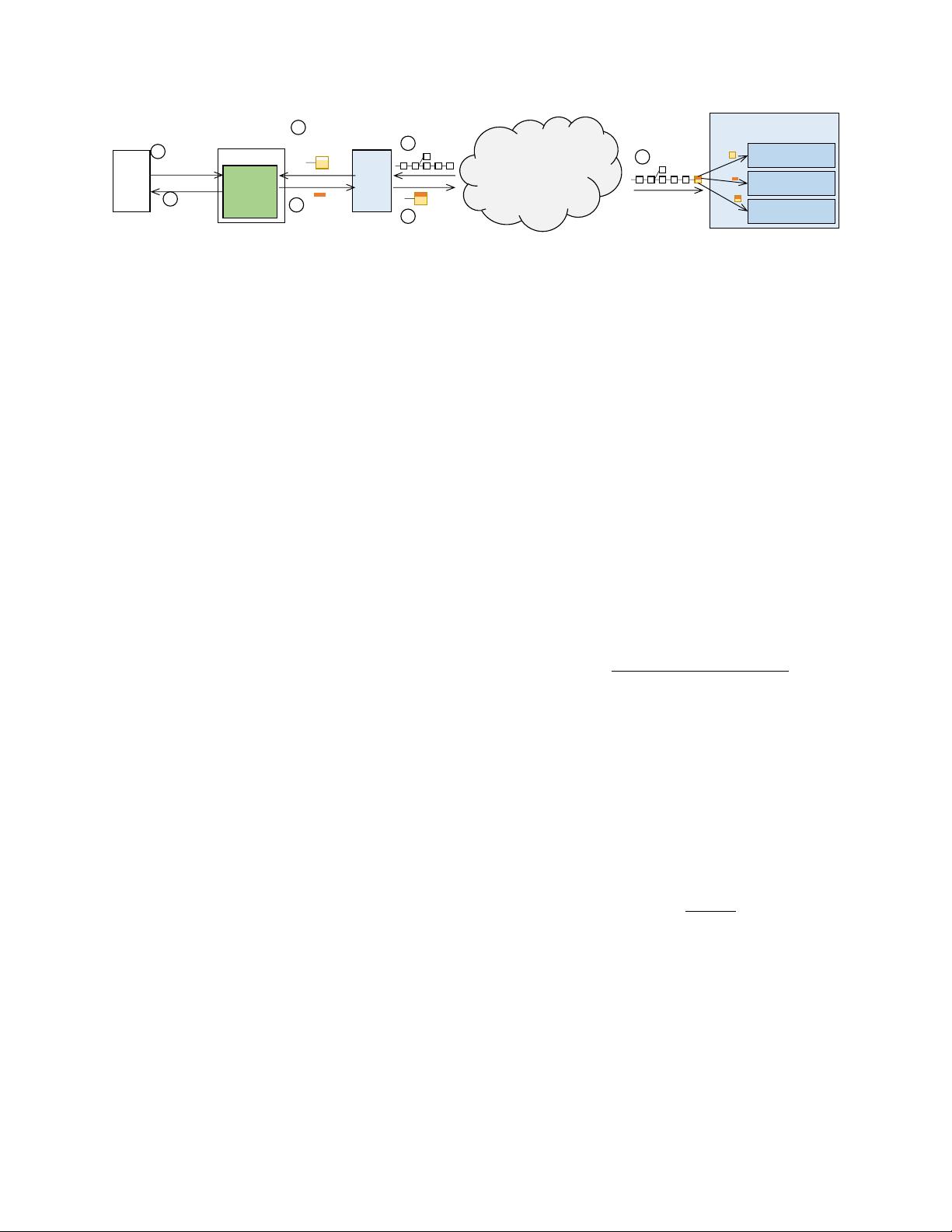
Figure 1: Architecture overview of REM
adversary’s ability to harvest blocks unfairly and mini-
mizes erroneous rejection of honestly mined blocks.
4.1 Threat Model and Definitions
4.1.1 Basic notation
To model block-acceptance policies, let M =
{m
1
,··· , m
n
} be the set of all miners, which we
assume to be static. (Miners can join and leave the
system; M includes all potential miners.) An adversary
A controls a static subset M
A
∈ M, where |M
A
| = k.
rate(m
i
) specifies the mining rate of m
i
, the number of
mining operations per unit time it performs.
We define a candidate block to be a tuple B = (t, m, d),
where t is a timestamp, m ∈ M the identity of the CPU
that mines the block, and d is the block difficulty. Diffi-
culty d is defined as the win probability per mining op-
eration in the underlying consensus protocol (e.g. a hash
in Bitcoin, a unit time of sleep in PoET, an instruction in
PoUW). B denotes the set of possible blocks B.
A blockchain is an ordered sequence of blocks. At
time τ, blockchain C(τ) is a sequence of accepted blocks
C(τ) = {B
1
,B
2
,...,B
n
} for some n. We drop τ where
its clear from context. We let r(τ) denote the number of
rejected blocks of honest miners, i.e., miners in M −M
A
,
in the history of C(τ). (Of course, r(τ) is not and indeed
cannot be recorded in a real blockchain system.) Let C
be the space of all possible blockchains C. Let C
m
denote
blockchain C restricted to blocks mined by miner m ∈M.
In REM, a blockchain-acceptance policy is used to de-
termine whether a block appears to come from a legiti-
mate miner (CPU that hasn’t been compromised).
Definition 1. (Blockchain-Acceptance Policy) A
blockchain-acceptance policy (or simply policy)
P : C×B → {reject,accept} is a function that takes as
input a blockchain and a proposed block, and outputs
whether the proposed block is legitimate.
4.1.2 Security and efficiency definitions
We model the consensus algorithm for the blockchain,
the adversary A, and honest miners respectively as
(ideal) programs prog
chain
, prog
A
, and prog
m
. Together,
they define what we call a security game S(P) for a par-
ticular policy P.
We define security games and their constituent pro-
grams formally in Appendix A.2. Where clear from con-
text in what follows, we use the notation S, rather than
S(P), i.e., omit P.
A security game S may itself be viewed as a proba-
bilistic algorithm. Thus we may treat the blockchain re-
sulting from execution of S for interval of time τ as a
random variable C
S
(τ).
Normalizing the revenue from mining a block to 1, we
define the payoff for a miner m for a given blockchain C
as π
m
(C) = |C
m
|.
An adversary A seeks to maximize payoffs for its min-
ers, as reflected in the following definition:
Definition 2. (Advantage of A). For a given security
game S, the advantage of A for time τ is:
Adv
S
A
(τ) =
E[π
ˆm
(C
S
(τ))]
max
m
j
∈M−M
A
E[π
m
j
(C
S
(τ))]
,
for any ˆm ∈M
A
. Note that E[π
ˆm
(C
S
(τ))] is equal for all
such ˆm, as they all use strategy Σ
A
and can emit blocks
as frequently as desired (ignoring rate( ˆm)).
A policy that keeps Adv
S
A
(τ) low is desirable, but
there’s a trade-off. A policy that rejects too many policies
incurs high waste, meaning that it rejects many blocks
from honest miners. We define waste as follows.
Definition 3. (Waste of a policy). For a given blockchain
C(τ) = {(B
1
,B
2
,...,B
n
)}, the waste is defined as
Waste(C(τ)) =
r(τ)
n + r(τ)
.
For security game S, the waste at time τ is defined as
Waste
S
(τ) = E[Waste(C
S
(τ))].
Our exploration of policies focuses critically on the
trade-offs between low Adv
S
A
(τ) and low Waste
S
(τ). To
illustrate the issue, we give a simple example in Ap-
pendix A.3 of a policy that allows any CPU to mine only
one block over its lifetime. As τ → ∞, it achieves the
optimal Adv
S
A
(τ) = 1, but at the cost of Waste
S
(τ) = 1,
i.e., 100% waste.
6

剩余25页未读,继续阅读

我就是月下
- 粉丝: 29
- 资源: 336
 我的内容管理
展开
我的内容管理
展开


最新资源
- Hadoop生态系统与MapReduce详解
- MDS系列三相整流桥模块技术规格与特性
- MFC编程:指针与句柄获取全面解析
- LM06:多模4G高速数据模块,支持GSM至TD-LTE
- 使用Gradle与Nexus构建私有仓库
- JAVA编程规范指南:命名规则与文件样式
- EMC VNX5500 存储系统日常维护指南
- 大数据驱动的互联网用户体验深度管理策略
- 改进型Booth算法:32位浮点阵列乘法器的高速设计与算法比较
- H3CNE网络认证重点知识整理
- Linux环境下MongoDB的详细安装教程
- 压缩文法的等价变换与多余规则删除
- BRMS入门指南:JBOSS安装与基础操作详解
- Win7环境下Android开发环境配置全攻略
- SHT10 C语言程序与LCD1602显示实例及精度校准
- 反垃圾邮件技术:现状与前景
资源上传下载、课程学习等过程中有任何疑问或建议,欢迎提出宝贵意见哦~我们会及时处理!
点击此处反馈


