避免错误因果关系与遗漏关联：从双变量时间序列推断耦合方向性

需积分: 3 49 浏览量更新于2024-07-31 收藏 310KB PDF 举报

"Directionality of coupling from bivariate time series: How to avoid false causalities and missed connections" 这篇文献探讨了从双变量时间序列中推断耦合方向性或因果关系时遇到的问题。在两个相互作用的系统中，正确识别因果关系至关重要，但这个过程可能受到多种因素和影响，导致测试敏感度降低或产生错误检测。作者米兰·帕卢斯(Milan Paluš)和马丁·韦杰梅尔卡(Martin Vejmelka)提出了解决这些问题的方法，以提高测试的敏感性和降低假阳性结果的比率。文章首先引出主题，指出合作行为在耦合复杂系统中的研究引起了理论和实验科学家的广泛关注，因为同步及相关现象不仅出现在物理系统中，也出现在许多生物系统中，如心脏系统的节律同步。在这些系统中，理解因果关系有助于揭示系统动态和功能的基础。接着，作者详细分析了可能导致推断方向性耦合问题的因素，包括但不限于数据质量、噪声干扰、非线性动力学、时间延迟以及样本大小等。在时间序列分析中，不充分考虑这些因素可能导致误判耦合的方向，甚至完全错过真实存在的连接。例如，非线性系统可能会隐藏真实的因果关系，使得传统的线性分析方法失效。为了提高测试敏感性，文献中提出了一些策略和方法，如使用适当的统计和计算技术来处理非线性数据，应用时间延迟嵌入来揭示隐藏的依赖关系，以及通过增加样本量来减小随机误差的影响。此外，文中还讨论了控制和校正共变量的重要性，因为共变量可以导致混淆，使得看起来像因果关系的关联实际上可能是由第三个未测量的变量引起的。在实际应用中，进行因果推断时应特别注意避免假阳性结果，这通常需要通过严格的统计检验和验证。文献中提到的策略包括使用多重检验校正以减少假阳性率，以及利用不同的因果推断方法进行一致性检查，如果多个独立的测试都指向相同的因果关系，那么这个结论就更可靠。该文对从双变量时间序列中推断耦合方向性和因果关系提供了深入的洞察，强调了正确识别这些关系的关键步骤和可能的陷阱。通过采用文中提出的建议和方法，研究人员能够更准确地解析复杂系统之间的交互，从而在物理、生物学和其他领域做出更有依据的科学发现。

0 0.2 0.4 0.6

0.1

(c)

COUPLING STRENGTH ε

i(X→Y), i(Y→X)

0 0.2 0.4 0.6

0.1

0.2

(a)

P(X→Y), P(Y→X)

0.1

0.2

0.1

0.2

0.3

0.4

(b)

S(X|Y), S(Y|X)

0.1

0.2

0.3

0.4

FIG. 2: (a) Cross-predictability P (X → Y ) (solid line) and

P (Y → X) (dashed line), (b) relative average distance of

the mutual nearest neighbours S

(k)

(Y|X) (solid line) and

(k)

(X|Y) (dashed line), and (c) coarse-grained transinfor-

mation rate i(X → Y ) (solid line) and i(Y → X) (dashed

line) for the unidirectionally coupled Henon system (3),(4),

as functions of the coupling strength ².

with that of Ref. [19]. Quian Quiroga et al. [19] ex-

plain that the higher-dimensional system (obtained by

the reconstruction from the time series {y

} which bears

information about both the coupled systems) is “more

active” than the lower-dimensional (autonomous, driv-

ing) system. Only the CTIR gives the same relation as

in the previous case: i(X → Y ) > i(Y → X) (Fig. 2c)

suggesting the fact that {X} inﬂuences {Y }, while {X}

evolves autonomously.

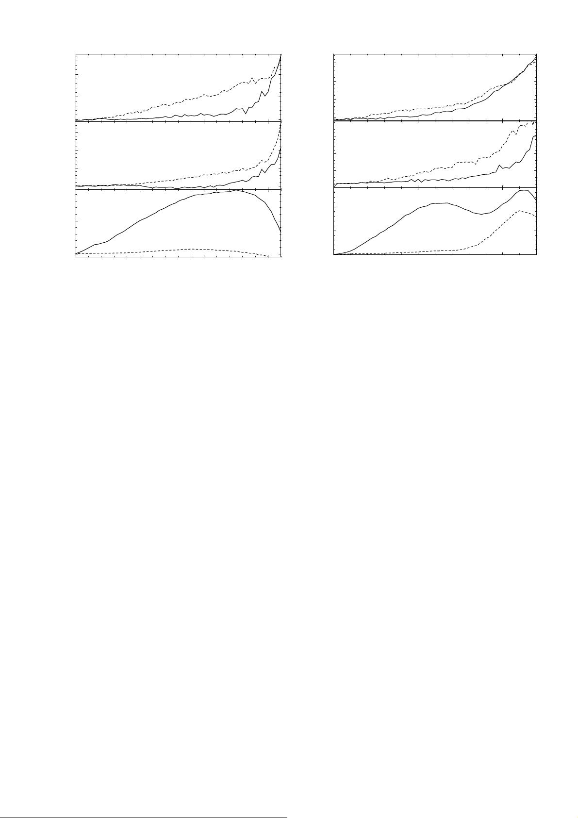
Figure 3 presents the analysis of the unidirectionally

coupled R¨ossler systems (5),(6). We can see that the

results are qualitatively the same as in the case of the

coupled Henon systems (Fig. 2), although these sys-

tems are more similar to the ﬁrst example of the cou-

pled R¨ossler-Lorenz systems. We can se that neither the

cross-predictability, nor the mutual nearest neighbours

statistics give consistent results when using three diﬀer-

ent examples of unidirectionally coupled systems. Only

the coarse-grained transinformation rate correctly iden-

tiﬁes the direction of the causal inﬂuence in the above

three examples as well as in many other systems of dif-

ferent origins tested by the authors.

In the above examples of unidirectionally coupled sys-

tems we could see that the used measures are generally

non-zero in both directions even before the systems be-

come synchronized and comparison of the values of such

measures does not always reﬂect the true causality given

by the unidirectional coupling of the studied systems.

The intuitively understandable implication lower predic-

0 0.05 0.1

0.05

0.1

(c)

COUPLING STRENGTH ε

i(X→Y), i(Y→X)

0 0.05 0.1

0.05

0.1

0.2

0.4

0.6

(a)

P(X→Y), P(Y→X)

0.2

0.4

0.6

0.01

0.02

0.03

(b)

S(X|Y), S(Y|X)

0.01

0.02

0.03

FIG. 3: (a) Cross-predictability P (X → Y ) (solid line) and

P (Y → X) (dashed line), (b) relative average distance of

the mutual nearest neighbours S

(k)

(Y|X) (solid line) and

(k)

(X|Y) (dashed line), and (c) coarse-grained transinfor-

mation rate i(X → Y ) (solid line) and i(Y → X) (dashed

line) for the unidirectionally coupled R¨ossler systems (5),(6),

as functions of the coupling strength ².

tion error (better predictability) => stronger dependence

cannot generally be applied for nonlinear systems. When

the coupling of the systems is weaker than that neces-

sary for the emergence of synchronization, as used in the

above examples, any smooth deterministic function be-

tween the states of the systems does not exist yet. How-

ever, there is already some statistical relation valid on

the coarse-grained description level. Although the deter-

ministic quantities are based on the existence of a smooth

functional relation, when estimated with ﬁnite precision

they usually give nonzero values inﬂuenced not only by

the existing statistical dependence but also by proper-

ties of the systems other then the coupling. It is there-

fore necessary to use quantities proposed for measur-

ing statistical dependence such as information-theoretic

measures which have solid mathematical background and

their properties have thoroughly been studied since their

introduction in 1948 [35].

III. DEPENDENCE MEASURES FROM

INFORMATION THEORY

In this Section we review basic measures from informa-

tion theory which we will need in further considerations.

More details can be found, e.g., in Refs. [35, 36]. Then

we will describe how these measures can help in inference

of causal relations or directionality of coupling.

Consider discrete random variables X and Y with sets

剩余15页未读，继续阅读

dsw3403221981

粉丝: 0
资源: 2

避免错误因果关系与遗漏关联：从双变量时间序列推断耦合方向性

directionality.rar_directionality_疵点_疵点纹理

Oracle sqldeveloper without jdk (win+linux)

matlabr2012b代码-microtubule-directionality:确定微管生长方向的MATLAB脚本

论文研究-Image Patch Clustering Based on Spectrum Structure and Directionality in Fourier Domain.pdf

retext-directionality:检测Retext中的方向性（从左到右，从右到左）

Kraken_Example_Text_Directionality:一个例子突出了 Kraken 中 Kraken 功能中 LTR 和 RTL 方向性的一种可能实现

On topology-related properties of abstract argumentation semantics. A correction and extension to Dynamics of argumentation systems: A division-based method

Subcycle Control of Electron-Electron Correlation in Double Ionization

Evaluation of Time Series Forecasting Models: In-depth Analysis of Key Metrics and Testing Methods

Unveiling the Autocorrelation Function in Practice: Mastering Time Series Periodicity and ...

最新资源