贝叶斯分析的弱信息先验选择：原因与实践

需积分: 50 74 浏览量更新于2024-07-17 收藏 1.3MB PDF 举报

"超越非信息先验：贝叶斯分析中选择弱信息性先验的原因和方法，Nathan P. Lemoine的论文，探讨了在贝叶斯统计中如何从非信息先验转向弱信息性先验的策略和理由。" 本文作者Nathan P. Lemoine指出，随着贝叶斯统计方法在生态学和进化生物学等领域中的广泛应用，如何有效地利用先验信息已成为一个关键问题。传统的非信息先验（uninformative priors）虽然在某些情况下提供了无偏的后验估计，但它们往往忽视了可用的背景知识，可能导致不准确或误导性的结果。因此，论文强调了采用弱信息性先验（weakly informative priors）的重要性。弱信息性先验是指那些对模型参数提供适度约束但又不会过度主导后验分布的先验。这类先验既反映了我们对参数的有限了解，又允许数据在分析中发挥主要作用。Lemoine在论文中详细阐述了选择和设计这类先验的哲学基础和实用技巧。首先，他解释了为什么应该使用弱信息性先验。在贝叶斯框架下，先验与数据一起决定后验分布，非信息先验可能导致后验分布过于广泛，使得结论的不确定性过大。而弱信息性先验能够利用领域知识缩小可能的参数范围，提高估计的精度和稳定性。其次，Lemoine讨论了选择弱信息性先验的方法。这包括但不限于：(1) 通过理论或实验研究来确定参数的合理范围；(2) 使用参考分布，如Jeffreys先验或Laplace规则；(3) 基于类似研究的结果设定先验；(4) 进行先验敏感性分析，确保选择的先验不影响主要结论。此外，论文还可能涵盖了如何评估和调整弱信息性先验的有效性，以及在实际数据分析中应用这些原则的案例研究。尽管未提供具体内容，但可以预期Lemoine会提供实际操作指导，帮助读者在自己的工作中实施这些方法。这篇论文为贝叶斯分析中的先验选择提供了一种更为细致入微的视角，强调了弱信息性先验在整合领域知识和数据之间的平衡作用，从而促进更可靠、更具解释力的统计推断。对于从事贝叶斯分析的科研人员来说，这是一份重要的参考资源，可以帮助他们更好地理解和应用先验信息。

Just as with linear regression, parameter estimates for mixed-effects models also converge for

maximum likelihood and noninformative Bayesian estimates. To illustrate, I simulated data from a multilevel

model with random-effects intercepts:

  

  

(6)





(7)



(8)

As before, I used 10,000 sets of randomly generated parameters [





, ,



] to simulate mixed-effects datasets

(see Appendix 2). For each dataset, I estimated fixed and random effects using mixed-effects models based on

maximum likelihood (statsmodels module) and Bayesian methods using noninformative priors (





, pystan module). The parameters were given informative priors of because of

the particular modeling approach used to impart numerical stability for the MCMC sampler (see Appendix 2).

As before, estimates of



were identical between maximum likelihood and Bayesian approaches with

noninformative priors (Fig. 3A). Noninformative priors also yielded identical estimates of





, with a few

exceptions where the maximum likelihood optimizer did not fully converge (Fig. 3B).

Because the same parameter estimates and statistical inferences result from both frequentist and

noninformative Bayesian analyses, both methods suffer from the same statistical issues. The “winner’s curse”

in particular has received considerable recent attention in both ecological and statistical literature [Button

et~al.(2013), Gelman and Carlin(2014), Lemoine et~al.(2016)]. The winner’s curse occurs when subsequent,

repeated experiments cannot replicate an initial significant finding [Ioannidis(2005)]. Statistical significance of

the original experiment occurred by chance, due to an overestimate of the true effect size (Type M error), which

caused a false positive (Type I error). Type I errors are ostensibly controlled by setting



, but the true

false positive rate (FPR) is the probability of a false positive given a significant result, which depends on

statistical power:





[Moyà1998), Appendix 3]. Similarly, the true positive rate,

known as the positive predictive value (PPV), is the probability of a true positive given a significant result:





[Button et~al.(2013), Heston and King(2017), Appendix 3]. PPV

and FPR both vary with statistical power; for studies with highly variable data, FPR can exceed 80% at low

sample sizes before converging to



at high sample sizes (Fig. 4). In other words, with noisy data, weak

effects, and small sample sizes, a statistically significant result is so unlikely that a significant result is more

likely to be a false positive than a true positive. This is true regardless of whether significance is calculated by

least squares, maximum likelihood, or Bayesian analyses with noninformative priors.

Accepted Article

Informative Priors

Many authors advocate the use of informative priors to alleviate problems like the winner’s curse that

arise from low statistical power. [Gelman and Hill(2007)] and [Gelman et~al.(2013)] state that noninformative

priors facilitate model development but should be substituted for informative priors during the final analyses.

More philosophically, both [Kruschke(2010)] and [Hobbs and Hooten(2015)] argue that current scientific

philosophy improperly idealizes science in vacuum, wherein only the data on hand are used to draw inferences;

science should instead utilize all available data. Despite these arguments, most textbooks on Bayesian data

analyses provide analytical and computational examples using noninformative priors, avoid making explicit

recommendations for informative priors, and do not illustrate how informative priors might affect results

[Gelman and Hill(2007), Kruschke(2010), Korner-Nievergelt et~al.(2015), but see ,Lemoine2016a]. Because

of the ambiguity surrounding prior choice and the pedagogy of Bayesian statistics emphasizing noninformative

priors, informative priors remain underutilized in ecological data analysis (Table 1).

This is unfortunate because many statistical issues like the winner’s curse can be mitigated via the use

of informative priors. Weakly informative priors serve as a method of statistical regularization, preventing the

winner’s curse by shrinking parameter estimates towards zero unless there is sufficiently strong evidence of a

large effect [McElreath(2015)]. Low-powered data result in larger shrinkage. In plainer words, large effect sizes

arising from limited sample sizes and noisy data are treated skeptically. Consider a few practical examples of

regularization. In the first example, imagine a -test comparing the mean of two groups. Standardizing the

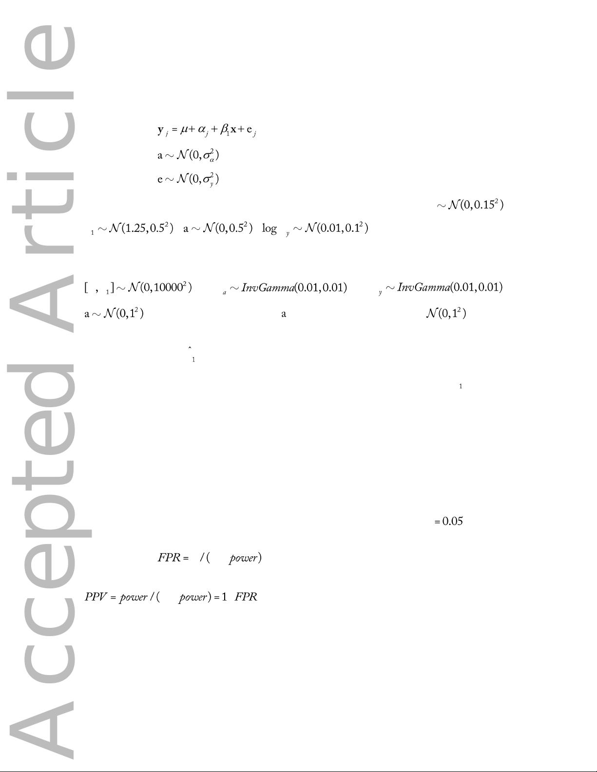
response variable and using a prior for the difference between groups states that effect sizes are

unlikely to be greater than one standard deviation of the response. This is an explicit acknowledgment that most

ecological effects are small [Mand Jennions(2002), Jennions and M(2003)] and that unrealistically large effects

in the data should be constrained unless supported by high statistical power (i.e. large sample sizes, low noise).

This effectively makes Bayesian analyses with weakly informative priors more conservative, but potentially

more accurate, than analyses based on noninformative priors. Weakly informative priors reduced statistical

power at sample sizes below 50, but also reduced Type I error rates nearly by half (Fig. 5, see Appendix 3). As

another example, I conducted 10,000 simulation experiments for an independent -test with a statistical power

of 0.2. For each simulation, I calculated the confidence interval for the effect size using both noninformative

and weakly informative priors. Under noninformative priors, the confidence interval failed to

include the true effect size in 3.59% of simulations, whereas the failure rate for weakly informative priors was

only 2.87%. Shrinkage can also mitigate the need for post-hoc corrections for multiple comparisons. [Gelman

et~al.(2012)] simulated data from multiple treatment groups with small effect sizes and conducted all pairwise

comparisons among groups. Out of 1,000 simulations, classical tests recorded at least one significant difference

47% of the time, whereas Bayesian analyses with shrinkage recorded at least one significant difference only 5%

of the time. However, Bayesian differences were 35% more accurate (i.e. correct sign) than classical analyses.

[Gelman et~al.(2012)] described the objective of regularization succinctly, as “the price to pay for more reliable

comparisons is to claim confidence in fewer of them”.

Accepted Article

剩余30页未读，继续阅读

loadbalancing

粉丝: 2
资源: 19

贝叶斯分析的弱信息先验选择：原因与实践

约束无信息先验贝叶斯神经网络学习

非确定先验信息的贝叶斯网结构学习方法 (2010年)

贝叶斯学习和增强：贝叶斯分类器和Adaboost算法的实现

BIGnav:贝叶斯信息增益（BIG）方法在多尺度导航中的核心功能

不确定性推理在糖果实验中的应用：贝叶斯分析与预测

贝叶斯方法入门：贝叶斯网络详解

贝叶斯方法：先验信息与后验分布详解

MCMC方法与WinBUGS：贝叶斯统计的收敛性诊断

模式识别基础：贝叶斯定理与特征选择

Python Pyautogui库详解：贝叶斯统计分析与指数分布

最新资源