
GANs for Anomaly Detection: a survey
Real / Fake
Input/Output
Conv
LeakyReLU
BatchNorm
ConvTranspose
ReLU Tanh Softmax
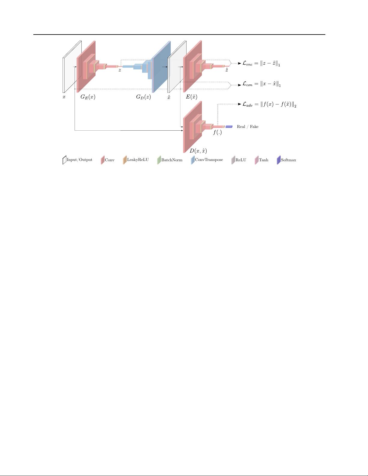
Figure 3. GANomaly architecture and loss functions from (Akcay et al., 2018).
et al. (2018). Their approach only needs a generator and a
discriminator as in a standard GAN architecture.
Generator network
The generator network consists of
three elements in series, an encoder
G
E
a decoder
G
D
(both assembling an autoencoder structure) and another en-
coder
E
. The architecture of the two encoders is the same.
G
E
takes in input an image
x
and outputs an encoded ver-
sion
z
of it. Hence,
z
is the input of
G
D
that outputs
ˆx
,
the reconstructed version of
x
. Finally,
ˆx
is given as an
input to the encoder
E
that produces
ˆz
. There are two main
contributions from this architecture. First, the operating
principle of the anomaly detection of this work lies in the
autoencoder structure. Given that we learn to encode nor-
mal (non-anomalous) data (producing
z
) and given that we
learn to generate normal data (
ˆx
) starting from the encoded
representation
z
, when the input data
x
is an anomaly its
reconstruction will be normal. Because the generator will al-
ways produce a non-anomalous image, the visual difference
between the input
x
and the produced
ˆx
will be high and in
particular will spatially highlight where the anomalies are
located. Second, the encoder
E
at the end of the generator
structure helps, during the training phase, to learn to encode
the images in order to have the best possible representation
of x that could lead to its reconstruction ˆx.
Discriminator network
The discriminator network
D
is
the other part of the whole architecture, and it is, with the
generator part, the other building block of the standard GAN
architecture. The discriminator, in the standard adversarial
training, is trained to discern between real and generated
data. When it is not able to discern among them, it means
that the generator produces realistic images. The generator
is continuously updated to fool the discriminator. Refer
to Figure 3 for a visual representation of the architecture
underpinning GANomaly.
The GANomaly architecture differs from AnoGAN (Schlegl
et al., 2017) and from EGBAD (Zenati et al., 2018). In
Figure 4 the three architectures are presented.
Beside these two networks, the other main contribution of
GANomaly is the introduction of the generator loss as the
sum of three different losses; the discriminator loss is the
classical discriminator GAN loss.
Generator loss
The objective function is formulated by
combining three loss functions, each of which optimizes a
different part of the whole architecture.
Adversarial Loss The adversarial loss it is chosen to be the
feature matching loss as introduced in Schlegl et al. (2017)
and pursued in Zenati et al. (2018):
L
adv
= E
x∼p
X
||f(x) − E
x∼p
X
f(G(x))||
2
,
(8)
where
f
is a layer of the discriminator
D
, used to extract
a feature representation of the input . Alternatively, binary
cross entropy loss can be used.
Contextual Loss Through the use of this loss the genera-
tor learns contextual information about the input data. As
shown in (Isola et al., 2016) the use of the
L
1
norm helps to
obtain better visual results:
L
con
= E
x∼p
X
||x − G(x)||
1
.
(9)
Encoder Loss This loss is used to let the generator network
learn how to best encode a normal (non-anomalous) image:
剩余15页未读,继续阅读


