Y. Ding et al. / Computer Methods and Programs in Biomedicine 156 (2018) 61–71 63
To measure the locality and the contribution of each data to x
c
,
a Gaussian kernel function is used to compute the weight w ( x, x
c
)
for each data point x ,
w (x, x
c
) ˆ = exp (−0 . 5 (x − x
c
)
T
D ( x − x
c
)) (1)
where D is a positive semi-definite distance metric, which deter-
mines the size and shape of the neighborhood contributing to the
local model.
Without loss of generality, the weights are required to normal-
ize data, which can be realized by subtracting the weighted mean
x or y from the data, where
¯
x
=
N
i =1
w ( x
i
, x
c
) x
i
N
i =1
w ( x
i
, x
c
)
¯
y
=
N
i =1
w ( x
i
, x
c
) y
i
N
i =1
w ( x
i
, x
c
) (2)
where x
i
indicates the i th sample in the dataset, and N is the num-
ber of data points.
During the whole procedure of nonlinear function approxima-
tion, the learning procedure involves automatically determining
the appropriate number of local models K ; parameters β of the hy-
per plane in each model; also the region of validity (called recep-
tive field, RF), parameterized as a distance metric D in a Gaussian
kernel.
Predictions
ˆ
y
k
(x ) (k = 1 , 2 , ··· , K) of each local linear model are
calculated for the given query point x
q
, and the final prediction
˜
y
q
of the learning system is the normalized weighted mean of all K
linear models [36] :
˜
y
q
=
K
k =1
w ( x
q
, x
k
c
)
y
k
K
k =1
w ( x
q
, x
k
c
) (3)
where
˜
y
q
denotes the global prediction of x
q
, x
k
c
indicates the cen-
ter point of the k th local model, and w ( x
q
, x
k
c
) is the weight be-
tween x
q
and x
k
c
.
In LWPR, updating the regression parameters is mainly realized
by using partial weighted partial least square algorithm (LWPLS),
of which the main idea is similar to the standard PLS except the
weight. The optimal projection direction is obtained by maximiz-
ing the covariance between input data and the regression residuals
in each step to find the optimal projection direction. For the k th
local model, the procedure of LWPLS is as follows [36] , and here
w
i
, ( i = 1, 2, , N ) indicates w ( x
i
, x
k
c
) for convenience, so does it in
the following sections.
The distance metric D and hence the locality of the receptive
fields can be learned for each local model individually by stochastic
gradient descent in a penalized leave-one-out cross validation cost
function [36] . D
def
is an original distance matrix, the initial number
of projection is set as R = 2.
When the first training data ( x
1
, y
1
) is joined, R = 2,
x
c
= x
1
, D = D
def
, ( D
def
is an original distance matrix) and a new
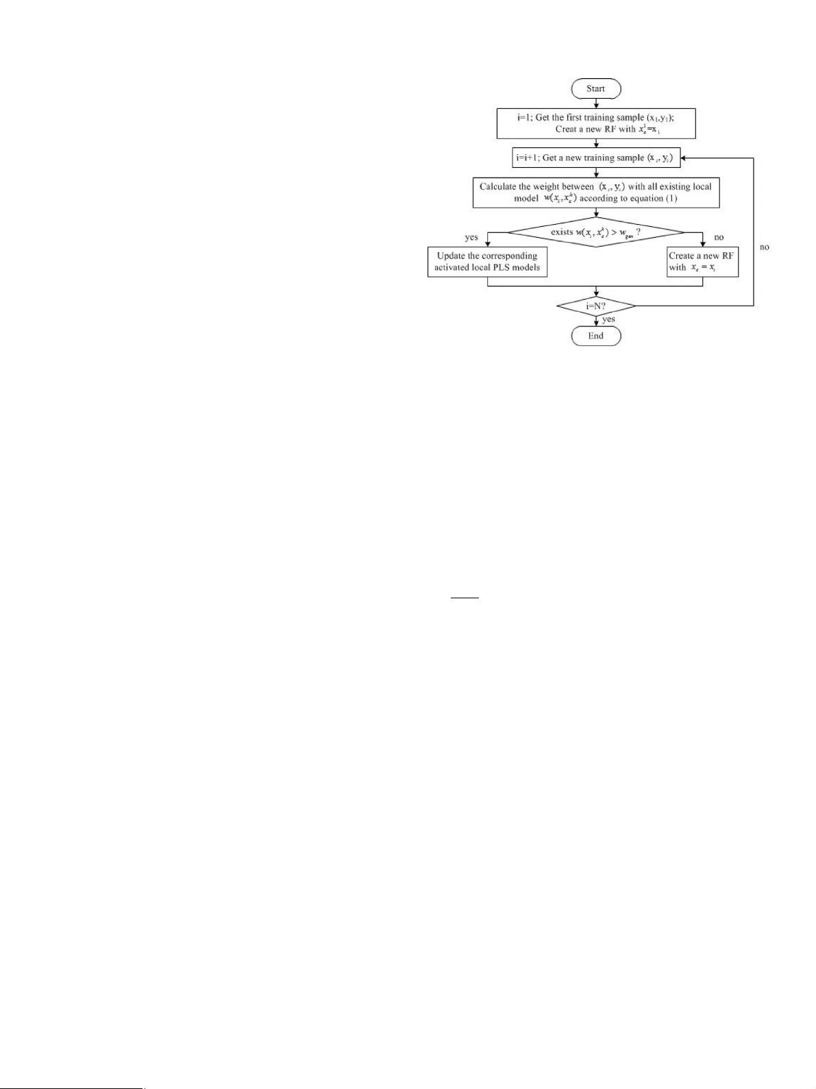
receptive field (RF, the region of validity) is created. Then with
the following training data, both the structure and the number
of local models are updated integrated with Gaussian kernel
weights, meanwhile the parameters R and D also changes. In
addition, a new RF will be created if all the weights are less than
a certain threshold w
gen
. For the sake of more clear illustration of
LWPR algorithm, Fig. 1 provides the simplified procedure of the
learning procedure, and a global model containing a series of local
models will be acquired in final. For a given query sample, the
corresponding global prediction output can be calculated by using
formula (3) .
Fig. 1. Simplified procedure of LWPR algorithm.
2.2. Principal component analysis
In the field of physiological processes, PCA is commonly used
for feature extraction and data compression instead of status mon-
itoring [37,38] . Its core idea is to transform multiple interrelated
variables into a few key independent components, which will de-
scribe the overall information, thus reducing the number of vari-
ables to be monitored. The procedure of simple PCA is as follows.
Assuming X
0
= ( x
ij
)
n × m
represents the original data matrix of
the normal process, where n denotes the measurement number, m
indicates the physical variables number, and n > m [39] . However,
the data matrix must be normalized to zero mean and unity vari-
ance, namely X , and the covariance matrix C is defined by
C =
1
n − 1
X
T
X
For the sake of extracting the main information, singular value
decomposition (SVD) is applied to the covariance matrix.
C = SS
T
=
S
pc
S
res
pc
0
0
res
S
pc
S
res
(4)
where S ∈ R
m × m
refers to the unit feature vectors of the covariance
matrix C , and S
pc
∈ R
m × r
corresponds to the eigenvalues sorted in
decreasing order ( λ
1
> λ
2
> λ
r
), while S
res
∈ R
m × ( m − r )
refers
to the remaining smaller eigenvalues ordered by λ
r + 1
> λ
r + 2
>
λ
m
, r denotes the number of exacted components, which can be
decided by several proposed approaches in the literature, such as
the SCREE procedure [22] , Cumulative Percent Variance (CPV) [40] .
Finally, X will be decomposed into the following two parts,
X =
ˆ
X +
˜
X = S
pc
S
T
pc
X + S
res
S
T
res
X (5)
where
ˆ
X abstracts the most information of the original variables,
while
˜
X , namely residual matrix, denotes the noise or uncertain
disturbance mostly when the measurements are fault free. Further-
more, the columns of S
pc
and S
res
tension into two orthogonal sub-
spaces, which refer to the principal component subspace and the
residual subspace, respectively.
Generally speaking, PCA uses two complementary statistics as
detection indices to measure the variation of the sample vectors’
projections in the principal component subspace and the residual
subspace, respectively, that is Hoteling’s T
2
[41] and squared pre-
diction error (SPE, also known as Q statistics) [42] , defined as
T
2
= X
T
S
pc
−1
pc
S
T
pc
X
SP E = X
T
S
res
S
T
res
X
(6)


