
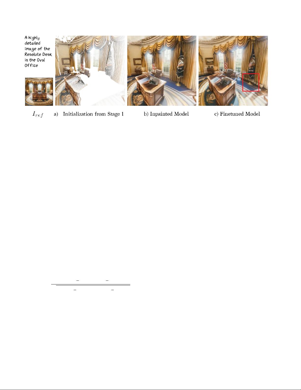
Figure 5. Progression of 3D Model after each stage. In this figure, we show how the 3D model changes after each stage in our pipeline.
As shown in a) Stage 1 (Sec. 4.1 creates a point cloud with many empty regions. In b), we show the subsequent inpainted model from
Stage 2 (Sec. 4.2). Finally, the fine-tuning stage (Sec. 4.4) refines b) to produce the final model, with greater cohesion and sharper detail.
dients outside the masked region.
4.3. Depth diffusion for text-to-3D
Recently, image-conditional depth diffusion models have
shown state-of-the-art results [29] for relative depth estima-
tion by finetuning a large-scale pre-trained RGB prior [51]
on depth datasets. In this section, we show how to distill the
knowledge from such methods for text-to-3D synthesis. We
consider a depth diffusion model ϵ
depth
which is conditioned
by images and text.
As mentioned in the previous section, during training,
we can draw samples ˆx using the inpainting diffusion model
ϵ
inpaint
applied to a noisy rendering of the current scene. Our
insight is to use these clean samples as the conditioning for
the depth diffusion model (shown in Fig. 4). Starting from
pure noise d
1
∼ N (0, I), we predict the normalized depth
using DDIM sampling [59]. We then compute the (negated)
Pearson Correlation between the rendered depth and sam-
pled depth:
L
depth
= −
P
(d
i
−
1
n
P
d
k
)(
ˆ
d
i
−
1
n
P
ˆ
d
k
)
q
P
(d
i
−
1
n
P
d
k
)
2
P
(
ˆ
d
i
−
1
n
P
ˆ
d
k
)
2
(6)
where d is the rendered depth from the 3DGS model and n
is the number of pixels.
4.4. Optimization and Finetuning
The final loss for the first training stage of our pipeline is
thus:
L
init
= L
inpaint
+ L
depth
. (7)
After training with this loss, we have a 3D scene that
roughly corresponds to the text prompt, but which may lack
cohesiveness between the reference image I
ref
and the in-
painted regions. To remedy this, we incorporate an addi-
tional lightweight finetuning phase. In this phase, we utilize
a vanilla text-to-image diffusion model ϵ
text
personalized for
the input image [15, 37, 48, 52]. We compute ˆx using the
same procedure as in Sec. 4.2, except with ϵ
text
. The loss
L
text
is the same as Eq. (5), except with the ˆz and ˆx sampled
with this finetuned diffusion model ϵ
text
.
To encourage sharp details in our model, we use a lower
noise strength than the inpainting stage and uniformly sam-
ple the timestep t within this limited range. We also propose
a novel sharpening procedure, which improves the sharp-
ness of our final 3D model. Instead of using ˆx to com-
pute the image-space diffusion loss introduced earlier, we
use S(ˆx), where S is a sharpening filter applied on samples
from the diffusion model. Finally, to encourage high opac-
ity points in our 3DGS model, we also add an opacity loss
L
opacity
per point that encourages the opacity of points to
reach either 0 or 1, inspired by the transmittance regularizer
used in Plenoxels [16].
The combined loss for the fine-tuning stage can be writ-
ten as:
L
finetune
= L
text
+ λ
opacity
L
opacity
, (8)
where λ
opacity
is a hyperparameter controlling the effect of
the opacity loss.
4.5. Implementation Details
Point Cloud Initialization. We implement the point cloud
initialization stage (Sec. 4.1) in Pytorch3D [49], with Stable
Diffusion [51] as our inpainting model. To lift the generated
samples to 3D, we use a high quality monocular depth esti-
6
剩余27页未读,继续阅读


人工智能_SYBH
- 粉丝: 4w+
- 资源: 220
 我的内容管理
收起
我的内容管理
收起
- 我的资源
快来上传第一个资源
 我的收益 登录查看自己的收益
 我的积分
登录查看自己的积分
我的积分
登录查看自己的积分
 我的C币
登录后查看C币余额
我的C币
登录后查看C币余额
 我的收藏
我的收藏  我的下载
我的下载  下载帮助
下载帮助

会员权益专享


最新资源
- GO婚礼设计创业计划:技术驱动的婚庆服务
- 微信行业发展现状及未来发展趋势分析
- 信息技术在教育中的融合与应用策略
- 微信小程序设计规范:友好、清晰的用户体验指南
- 联鼎医疗:三级甲等医院全面容灾备份方案设计
- 构建数据指标体系:电商、社区、金融APP案例分析
- 信息技术:六年级学生制作多媒体配乐古诗教程
- 六年级学生PowerPoint音乐动画实战:制作配乐古诗演示
- 信息技术教学设计:特点与策略
- Word中制作课程表:信息技术教学设计
- Word教学:制作课程表,掌握表格基础知识
- 信息技术教研活动年度总结与成果
- 香格里拉旅游网设计解读:机遇与挑战并存
- 助理电子商务师模拟试题:设计与技术详解
- 计算机网络技术专业教学资源库建设与深圳IT产业结合
- 微信小程序开发:网络与媒体API详解
资源上传下载、课程学习等过程中有任何疑问或建议,欢迎提出宝贵意见哦~我们会及时处理!
点击此处反馈


