Algorithm 1: SCOA
Input: The set of queries Q = {q
1
, q
2
, ..., q
m
};
The initial column order S
0
= {c
1
, c
2
, ..., c
n
}
Output: The optimized column order S;
1 S := S
0
, e := Cost(Q, S
0
), t := t
0
;
2 for k := 1 to k
max
do
3 t := T emperature(t, cooling_rate);
4 S
0
:= Neighbor(S);
5 e
0
:= Cost(Q, S
0
);
6 if (e
0
< e)||(exp((e − e
0
)/t) > random(0, 1)) then
7 S := S
0
;
8 e := e
0
;
9 return S;
proposed in [35]. The Temperature function is the core function of
the annealing schedule. In this algorithm, the temperature shrinks at
a rate of
(1 − cooling_rate)
. Function Neighbor(S) is to generate
a candidate neighboring state from the current state
S
, achieved
by swapping the positions of two randomly picked columns in
S
.
1
Parameter settings of SCOA are discussed in Appendix C.
3.3 Incremental Computation of Seek Cost
When the access pattern of a query follows the global column
order (as adopted by existing systems such as HDFS), we can incre-
mentally compute the seek cost of a query to speed up SCOA, given
that a neighboring state
S
0
is derived from the current state
S
by
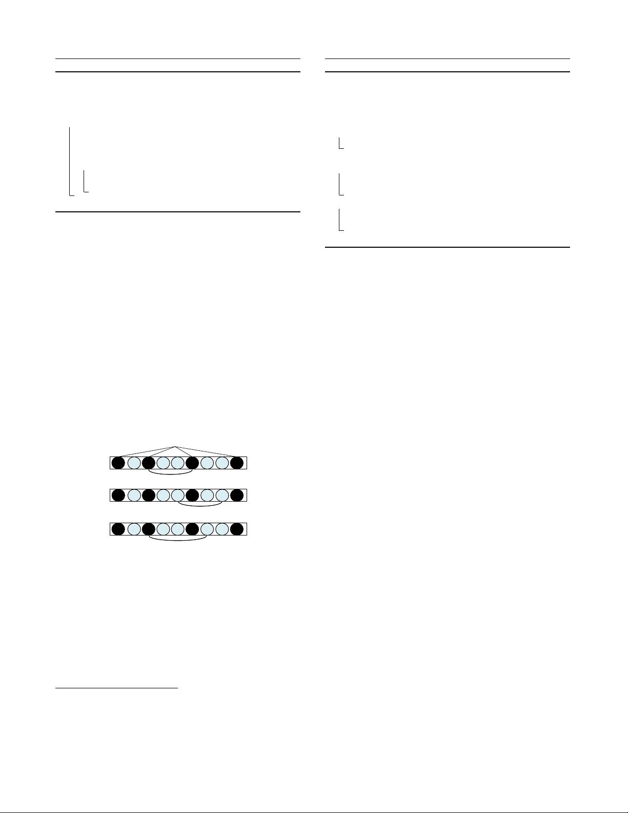
randomly swapping two columns. Consider the example in Figure 2.
Query
q
accesses 4 columns
C
q
= {c
4
, c
2
, c
6
, c
8
}
. When deriving
a new state by swapping two columns in
C
q
(e.g.,
c
2
and
c
6
in
Figure 2(a)), the seek cost of this query clearly remains unchanged
(both equal to
f(s(c
5
)) + f(s(c
1
) + s(c
3
)) + f(s(c
7
) + s(c
9
))
,
for reading a row group).
c
2
c
1
c
6
c
9
c
8
c
4
c
5
c
3
c
7
q
(a) Swap c
2
and c
6
(b) Swap c
3
and c
9
c
2
c
1
c
6
c
9
c
8
c
4
c
5
c
3
c
7
(c) Swap c
2
and c
7
c
2
c
1
c
6
c
9
c
8
c
4
c
5
c
3
c
7
Figure 2: Three cases of the delta query cost
A more complex case occurs when neither of the two swapped
columns is accessed by the query
q
(e.g.,
c
3
and
c
9
in Figure 2(b)).
The pseudo code for handling this case is presented in Algorithm 2.
The
SeekCost2ndCase
function takes as input the current state
S
and two swapped columns
c
x
and
c
y
, and outputs the seek cost of
the neighboring state
S
0
for
q
. Let
suc(c
i
)
be the first succeeding
column of
c
i
in
C
q
, and
pre(c
i
)
be first preceding column of
c
i
in
C
q
. For example, in Figure 2,
suc(c
1
) = c
6
and
pre(c
1
) = c
2
.
According to Algorithm 2, it is clear that
Cost(q, S
0
) = Cost(q, S)
if
suc(c
x
) = suc(c
y
)
. Otherwise, at most two terms in Equation 2
1
We have also tested various other neighboring state selection heuris-
tics, including substantially more complicated ones. However, none
of them outperformed the simple ‘column-swap’ heuristic. For the
sake of simplicity, we thus limit ourselves to the presentation of this
most basic version of the algorithm.
Algorithm 2: SeekCost2ndCase
Input: A query q and sorted set C
q
;
Current column order S, and its seek cost Cost(q, S);
Two swapped columns, c
x
/∈ C
q
and c
y
/∈ C
q
.
Output: The seek cost of the neighboring state S
0
,
Cost(q, S
0
)
1 if suc(c
x
) = suc(c
y
) then
2 return Cost(q, S);
3 delta := 0;
4 if pre(c
x
) 6= null and suc(c
x
) 6= null then
5 delta −= f (b(suc(c
x
)) − e(pre(c
x
)));
6 delta += f(b(suc(c
x
)) − e(pre(c
x
)) − s(c
x
) + s(c
y
))
;
7 if pre(c
y
) 6= null and suc(c
y
) 6= null then
8 delta −= f (b(suc(c
y
)) − e(pre(c
y
)));
9 delta += f (b(suc(c
y
)) − e(pre(c
y
)) − s(c
y
) + s(c
x
));
10 return Cost(q, S) + delta;
will be affected and it will be updated according to Lines 4-6 and
Lines 7-9, respectively.
The last case occurs when exactly one swapped column is ac-
cessed by
q
(e.g. Figure 2(c)), which can be handled in a similar
way to Algorithm 2. An important difference from the previous two
cases is that
C
q
will be updated if the SA algorithm accepts this
neighboring state S
0
.
Time Complexity.
To maintain the sorted set
C
q
efficiently,
we use a binary balanced search tree to insert, remove and query
preceding and succeeding elements. All these operations run in
O(log R)
time. The overall time complexity of computing seek
costs is
O(|Q|· log R)
, where
R
is the average number of columns
accessed by a query. Compared to the naive approach of sorting all
the columns for every new ordering, this incremental approach is
R
times faster. On the production data we tested,
R
is 32 and SCOA
with incremental seek cost computation only requires a few minutes
to converge.
Besides simulated annealing (SA), we have tried several other
meta heuristics. Particularly, we have also tried to apply genetic
algorithm (GA) [37, 51] in Appendix D and AutoPart [41] algorithm
in Appendix E. Results show that SA performs much better.
4. STORAGE CONSTRAINED COLUMN DU-
PLICATION
Suppose we have extra storage headroom, we may be able to
further reduce the overall seek cost by duplicating some popular
columns and inserting them into carefully selected positions within
the derived column orders. Consider the simple example in Figure
3. In Fig. 3(a), the seek cost of both
q
1
and
q
2
is 0 while the seek
cost of
q
3
is
f(s(c
3
) + s(c
6
))
(Note that the initial seek cost
can
be ignored as it is constant). In Fig. 3(b), however, if we duplicate
c
1
, insert it between
c
6
and
c
7
, and let
q
3
access the new replica of
c
1
, the seek cost of all three queries becomes 0.
We formally define the column duplication problem as follows.
DEFINITION 7 (COLUMN DUPLICATION PROBLEM).
Given a workload
Q
and the storage headroom
H
, identify a set of
duplicated columns with an ordering strategy
S
D
such that 1) the
total size of duplicated columns is not greater than
H
and 2) the
seek cost of Q is minimized.
In this section, we first introduce the basic idea of the duplication
process in Section 4.1 and then provide details of how to optimize it
in Section 4.2.


