216
217
218
219
220
221
222
223
224
225
226
227
228
229
230
231
232
233
234
235
236
237
238
239
240
241
242
243
244
245
246
247
248
249
250
251
252
253
254
255
256
257
258
259
260
261
262
263
264
265
266
267
268
269
270
271
272
273
274
275
276
277
278
279
280
281
282
283
284
285
286
287
288
289
290
291
292
293
294
295
296
297
298
299
300
301
302
303
304
305
306
307
308
309
310
311
312
313
314
315
316
317
318
319
320
321
322
323
CVPR
#****
CVPR
#****
CVPR 2019 Submission #****. CONFIDENTIAL REVIEW COPY. DO NOT DISTRIBUTE.
We can see that (2) degenerates (1) when K =1and Q
1
is the identical function. But the difference with NNM is
that MCMT looks for the low-rank solution under linear
transformations rather than the matrix itself. It implies that
(2) can be used to complete the matrix that has a high-rank
structure.
Comparison with matrix sensing. Matrix sensing is to re-
cover the original matrix from the Gaussian measurements.
The model is formalized as
min
X2R
m
1
⇥m
2
kXk
⇤
,s.t.kQ(X) Q ( Y) k
F
< , (3)
where the entries of Q follows the i.i.d. Gaussian distribu-
tion. Compared with (2), (3) only consider the linear trans-
formation Q in the constraint term. Furthermore, matrix
sensing also exploit the low-rank structure of the original
matrix like NNM, while MCMT takes into account the ad-
ditional low-rank structures under linear transformations.
comparison with CTD. As mentioned in the related
works, CTD is to seek for the approximation of a tensor
with multi-linear low-rank structures. For a K-th order ten-
sor and its perturbed variant Y, CTD is given by [?]
min
X2R
m
1
⇥m
2
X
i2[K]
[X ]
(i)
⇤
,
s.t. kP
⌦
(X ) P
⌦
(Y)k
F
< ,
(4)
where [X ]
(i)
denotes unfolding the tensor X along i-th
order [?]. Due to the fact that the unfolding operations
are linear functions, (4) is a special case of MCMT when
Q
i
(·)=[· ]
(i)
. It is worthwhile to mention that tensor
unfolding only rearrange the tensor into different shapes,
but MCMT can use more general linear functions like re-
sampling, rotation and stretching in the linear space to dig
more structures of the matrix.
2.4. Examples of Q
i
in MCMT
In MCMT, the linear transformations Q
i
, 8 i can be used
to formulate specific operations in various CV applications.
Here we show some examples.
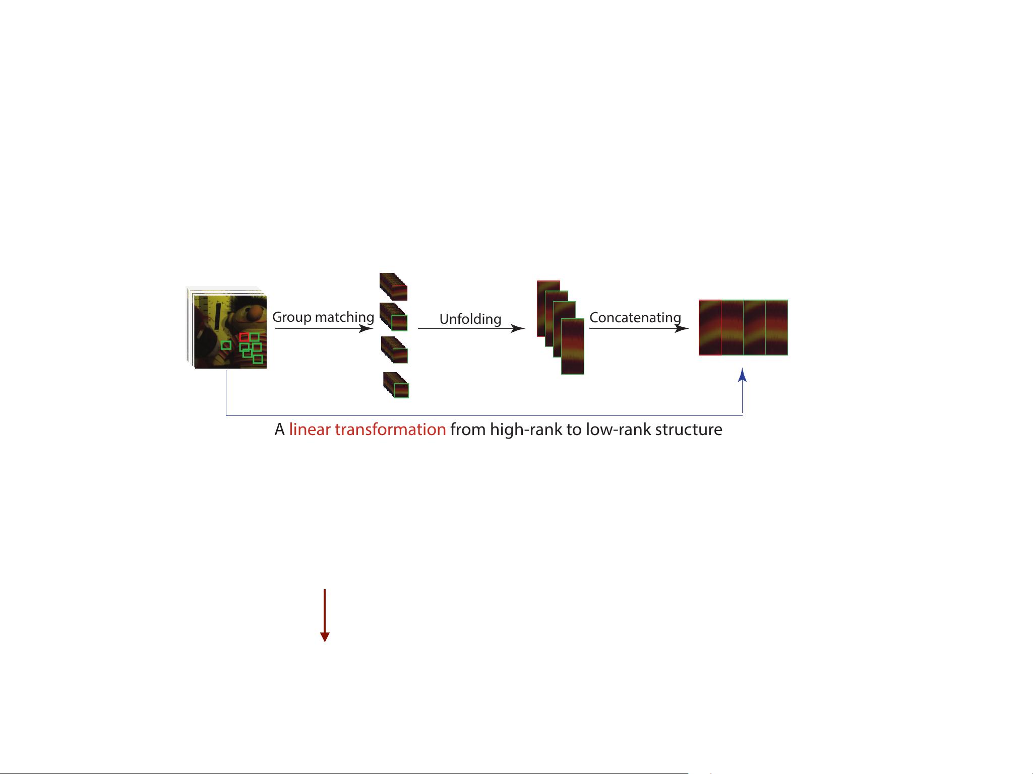
Example 1 (non-local image restoration). To exploit the
non-local similarity of the images, the methods usually split
the whole matrix into many “non-local groups”, and each
group is a concatenation of similar patches of the image.
We can see that such grouping operation is mathematically
a down-sampling (definitely linear) function from the image
to the non-local group. Therefore, each Q
i
(X),i 2 [K] in
(2) corresponds to K non-local groups, and solving (2) is
to find the optimal low-rank approximation for each non-
local group and then merge the approximations back to the
global image.
Example 2 (occlusion removal). In the occlusion removal
problem, the original image is generally covered by some
other objects, and the aim of this application is to recover
the hidden part of the image. To solve this problem, the pre-
vious study [?] assume that both the original image and the
covered part have the low-rank structures. By using MCMT,
we can specify K =2, set Q
1
to be the identical function
to catch the low-rank structure of the image, and set Q
2
to
obtain the covered sub-image with the low-rank structures.
Besides these examples, we can also specify Q
i
as the
2-D wavelet filters to catch the short-term fluctuation of
the image under multiple resolutions or even random shuf-
fling [?].
3. Identifiablity
One of the advantage of LRMC is that the completion
performance is theoretically guaranteed. In this section,
we theoretically analyze the reconstruction error of MCMT,
and reveal what conditions Q
i
, 8 i should satisfy for exact
recovery.
In the rest of this section, we first establish an upper
bound of MCMT under a single linear transformation, i.e.
K =1. After that, we extend the results to the case of
multiple transformations.
3.1. Single linear transformation
Assume that M
0
2 R
m
1
⇥m
2
denotes the “true” ma-
trix that we want to recover, and its rank equals R . The
noised variant of M
0
is generated by Y = M
0
+ H where
the entries of H obey the i.i.d. Gaussian distribution, i.e.
H(i, j) ⇠ N(0,
2
) for all i 2 [m
1
],j 2 [m
2
]. With the
single linear transformation, we simplify (2) as
min
X2R
m
1
⇥m
2
kQ(X)k
⇤
s.t. kP
⌦
(X) P
⌦
(Y)k
F
,
(5)
where the subscript of Q 2 R
m
1
⇥m
2
⇥n
1
⇥n
2
is removed
for brevity. Let Q(M
0
)=UDV
>
be the truncated
singular value decomposition (SVD), in which only the
singular vectors with respect to non-zero singular val-
ues are kept. Furthermore, we define a linear space
T =
n
UX
>
+ YV
>
|X 2 R
n
1
⇥R
, Y 2 R
n
2
⇥R
o
, which
reflects the properties of the neighborhood around M
0
. Let
T
?
denote the orthogonal complement to T. Based on the
dual theory, we define the dual certificate for unique solu-
tion of (5) as follow:
Definition 2 (Dual certificate). A matrix ⇤ 2 R
m
1
⇥m
2
is
defined as a dual certificate of (5), if P
⌦
(⇤)=⇤ and ⇤
can be decomposed as
⇤ = Q
?
⇣
UV
>
+ R
⇤
⌘
, (6)
where R
⇤
= P
T
?
(⇤), P
T
?
denotes the projection to T
?
and kR
⇤
k
2
1.
3


