数学模型与应用：微分方程与线性代数

需积分: 50 2 浏览量更新于2024-07-17 1 收藏 23.7MB PDF 举报

"Differential Equations and Linear Algebra, 4th Edition" 是一本由C. Henry Edwards、David E. Penney和David Calvis合著的教材，适用于大学的微分方程和线性代数课程。这本书结合了基础微分方程和线性代数的核心概念，通过现实世界的应用进行数学建模。第四版在图形、示例、问题和应用中增添了新的计算和定性元素，并提供了一个包含扩展应用和编程工具的网站。本书内容包括： 1. 首阶微分方程：介绍基本的微分方程解法。 2. 数学模型与数值方法：探讨如何用微分方程来模拟真实世界的系统。 3. 线性系统与矩阵：讨论线性系统的解法以及矩阵的基本操作。 4. 向量空间：深入理解向量空间的性质和运算。 5. 更高阶线性微分方程：研究一阶以上微分方程的解法。 6. 特征值与特征向量：探讨线性变换的特性。 7. 线性微分方程组：处理多变量线性系统的动态行为。 8. 矩阵指数方法：利用矩阵指数解决线性系统。 9. 非线性系统与现象：探讨非线性方程组的解法。 10. 拉普拉斯变换方法：利用拉普拉斯变换求解微分方程。 11. 功率级数方法：使用幂级数解微分方程。此外，书后还有进一步学习的参考资料，附录涵盖了解的存在性和唯一性理论以及行列式理论。本书的特点是其丰富的现实世界应用，强调数学模型的建立，以及对定性和计算方法的平衡处理。它还提供了精心设计的问题集，旨在帮助学生将理论知识应用于实践。通过使用这本教材，学生不仅能掌握微分方程和线性代数的基础，还能了解这些数学工具如何在工程、物理、经济等领域解决问题。该版本更新了教学内容，增加了新的计算和定性元素，使学生能够更好地理解和应用这些概念。此外，配套的扩展应用网站提供了额外的案例和编程工具，增强了学习体验，帮助学生深化理解并提升技能。

First-Order

Differential Equations

1.1 Differential Equations and Mathematical Models

he laws of the universe are written in the language of mathematics. Algebra

is sufﬁcient to solve many static problems, but the most interesting natural

phenomena involve change and are described by equations that relate changing

quantities.

Because the derivative dx=dt D f

.t/ of the function f is the rate at which

the quantity x D f .t/ is changing with respect to the independent variable t, it

is natural that equations involving derivatives are frequently used to describe the

changing universe. An equation relating an unknown function and one or more of

its derivatives is called a differential equation.

Example 1 The differential equation

D x

C t

involves both the unknown function x.t / and its ﬁrst derivative x

.t/ Ddx=dt . The differential

equation

C 3

C 7y D 0

involves the unknown function y of the independent variable x and the ﬁrst two derivatives

and y

of y.

The study of differential equations has three principal goals:

1. To discover the differential equation that describes a speciﬁed physical

situation.

2. To ﬁnd—either exactly or approximately—the appropriate solution of that

equation.

3. To interpret the solution that is found.

In algebra, we typically seek the unknown numbers that satisfy an equation

such as x

C7x

11x C41 D 0. By contrast, in solving a differential equation, we

2 Chapter 1 First-Order Differential Equations

are challenged to ﬁnd the unknown functions y D y.x/ for which an identity such

as y

.x/ D 2xy.x/—that is, the differential equation

D 2xy

—holds on some interval of real numbers. Ordinarily, we will want to ﬁnd all

solutions of the differential equation, if possible.

Example 2 If C is a constant and

y.x/ D C e

; (1)

then

D C



2xe



D .2x/





D 2xy:

Thus every function y.x/ of the form in Eq. (1) satisﬁes—and thus is a solution of—the

differential equation

D 2xy (2)

for all x. In particular, Eq. (1) deﬁnes an inﬁnite family of different solutions of this differen-

tial equation, one for each choice of the arbitrary constant C . By the method of separation of

variables (Section 1.4) it can be shown that every solution of the differential equation in (2)

is of the form in Eq. (1).

Differential Equations and Mathematical Models

The following three examples illustrate the process of translating scientiﬁc laws and

principles into differential equations. In each of these examples the independent

variable is time t, but we will see numerous examples in which some quantity other

than time is the independent variable.

Example 3 Rate of cooling Newton’s law of cooling may be stated in this way: The time rate of change

(the rate of change with respect to time t) of the temperature T .t/ of a body is proportional

to the difference between T and the temperature A of the surrounding medium (Fig. 1.1.1).

That is,

d T

D k.T  A/; (3)

where k is a positive constant. Observe that if T > A, then d T=dt < 0, so the temperature is

a decreasing function of t and the body is cooling. But if T < A, then d T=dt > 0, so that T

is increasing.

Thus the physical law is translated into a differential equation. If we are given the

values of k and A, we should be able to ﬁnd an explicit formula for T .t/, and then—with the

aid of this formula—we can predict the future temperature of the body.

Temperature T

Temperature A

FIGURE 1.1.1. Newton’s law of

cooling, Eq. (3), describes the cooling

of a hot rock in water.

Example 4 Draining tank Torricelli’s law implies that the time rate of change of the volume V of

water in a draining tank (Fig. 1.1.2) is proportional to the square root of the depth y of water

in the tank:

D k

y; (4)

where k is a constant. If the tank is a cylinder with vertical sides and cross-sectional area A,

then V D Ay, so dV=dt D A  .dy=dt/. In this case Eq. (4) takes the form

h

y; (

where h D k=A is a constant.

Volume V

FIGURE 1.1.2. T

orricelli’s law of

draining, Eq. (4), describes the

draining of a water tank.

1.1 Differential Equations and Mathematical Models 3

Example 5 Population growth The time rate of change of a population P .t / with constant birth and

death rates is, in many simple cases, proportional to the size of the population. That is,

D kP; (6)

where k is the constant of proportionality.

Let us discuss Example 5 further. Note ﬁrst that each function of the form

P .t / D Ce

(7)

is a solution of the differential equation

D kP

in (6). We verify this assertion as follows:

.t/ D C ke

D k





D kP.t/

for all real numbers t. Because substitution of each function of the form given in

(7) into Eq. (6) produces an identity, all such functions are solutions of Eq. (6).

Thus, even if the value of the constant k is known, the differential equation

dP=dt D kP has inﬁnitely many different solutions of the form P.t/ D Ce

, one for

each choice of the “arbitrary” constant C . This is typical of differential equations.

It is also fortunate, because it may allow us to use additional information to select

from among all these solutions a particular one that ﬁts the situation under study.

Example 6 Population growth Suppose that P .t/ D C e

is the population of a colony of bacteria at

time t, that the population at time t D 0 (hours, h) was 1000, and that the population doubled

after 1 h. This additional information about P .t / yields the following equations:

1000 D P .0/ D C e

D C;

2000 D P .1/ D C e

It follows that C D 1000 and that e

D 2, so k D ln 2  0:693147. With this value of k the

differential equation in (6) is

D .ln 2/P  .0:693147/P:

Substitution of k D ln 2 and C D 1000 in Eq. (7) yields the particular solution

P .t/ D 1000e

.ln 2/t

D 1000.e

ln 2

D 1000  2

(because e

ln 2

D 2)

that satisﬁes the given conditions. We can use this particular solution to predict future popu-

lations of the bacteria colony. For instance, the predicted number of bacteria in the population

after one and a half hours (when t D 1:5) is

P .1:5/ D 1000  2

3=2

 2828:

The condition P .0/ D1000 in Example 6 is called an initial condition because

we frequently write differential equations for which t D 0 is the “starting time.”

Figure 1.1.3 shows several different graphs of the form P.t/ D Ce

with k D ln 2.

The graphs of all the inﬁnitely many solutions of dP=dt D kP in fact ﬁll the entire

two-dimensional plane, and no two intersect. Moreover, the selection of any one

point P

on the P -axis amounts to a determination of P .0/. Because exactly one

solution passes through each such point, we see in this case that an initial condition

P .0/ D P

determines a unique solution agreeing with the given data.

0 1 2 3

–2

–1

–4

–2

–6

–8

C = 12

C = 6 C = 3

C = –6

C =

C = –

C = 1

C = –1

C = –3C = –12

FIGURE 1.1.3. G

raphs of

P .t/ D Ce

with k D ln 2.

4 Chapter 1 First-Order Differential Equations

Mathematical Models

Our brief discussion of population growth in Examples 5 and 6 illustrates the crucial

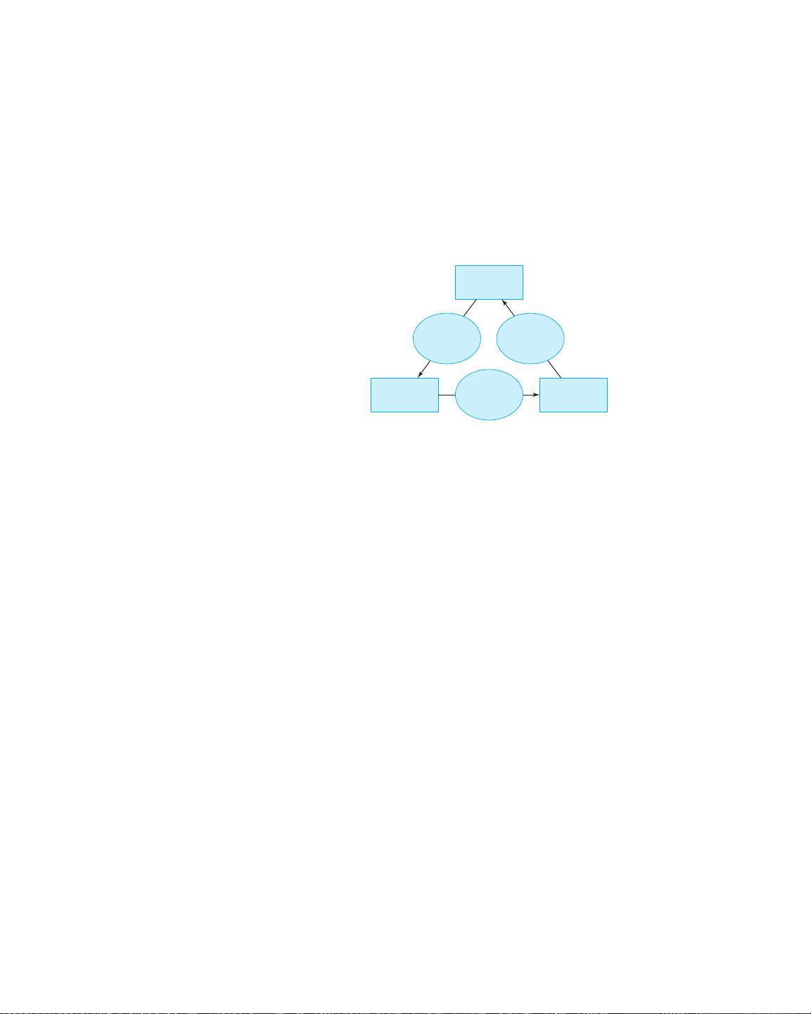
process of mathematical modeling (Fig. 1.1.4), which involves the following:

1. The formulation of a real-world problem in mathematical terms; that is, the

construction of a mathematical model.

2. The analysis or solution of the resulting mathematical problem.

3. The interpretation of the mathematical results in the context of the original

real-world situation—for example, answering the question originally posed.

Real-world

situation

Mathematical

model

Mathematical

results

Mathematical

analysis

Formulation Interpretation

FIGURE 1.1.4. T

he process of mathematical modeling.

In the population example, the real-world problem is that of determining the

population at some future time. A mathematical model consists of a list of vari-

ables (P and t) that describe the given situation, together with one or more equations

relating these variables (dP=dt D kP , P .0/ D P

) that are known or are assumed to

hold. The mathematical analysis consists of solving these equations (here, for P as

a function of t). Finally, we apply these mathematical results to attempt to answer

the original real-world question.

As an example of this process, think of ﬁrst formulating the mathematical

model consisting of the equations dP=dt D kP , P .0/ D 1000, describing the bac-

teria population of Example 6. Then our mathematical analysis there consisted of

solving for the solution function P .t/ D 1000e

.ln 2/t

D 1000  2

as our mathemat-

ical result. For an interpretation in terms of our real-world situation—the actual

bacteria population—we substituted t D 1:5 to obtain the predicted population of

P .1:5/  2828 bacteria after 1.5 hours. If, for instance, the bacteria population is

growing under ideal conditions of unlimited space and food supply, our prediction

may be quite accurate, in which case we conclude that the mathematical model is

adequate for studying this particular population.

On the other hand, it may turn out that no solution of the selected differential

equation accurately ﬁts the actual population we’re studying. For instance, for no

choice of the constants C and k does the solution P.t/ D C e

in Eq. (7) accurately

describe the actual growth of the human population of the world over the past few

centuries. We must conclude that the differential equation dP=dt DkP is inadequate

for modeling the world population—which in recent decades has “leveled off” as

compared with the steeply climbing graphs in the upper half (P > 0) of Fig. 1.1.3.

With sufﬁcient insight, we might formulate a new mathematical model including

a perhaps more complicated differential equation, one that takes into account such

factors as a limited food supply and the effect of increased population on birth and

death rates. With the formulation of this new mathematical model, we may attempt

to traverse once again the diagram of Fig. 1.1.4 in a counterclockwise manner. If

we can solve the new differential equation, we get new solution functions to com-

1.1 Differential Equations and Mathematical Models 5

pare with the real-world population. Indeed, a successful population analysis may

require reﬁning the mathematical model still further as it is repeatedly measured

against real-world experience.

But in Example 6 we simply ignored any complicating factors that might af-

fect our bacteria population. This made the mathematical analysis quite simple,

perhaps unrealistically so. A satisfactory mathematical model is subject to two con-

tradictory requirements: It must be sufﬁciently detailed to represent the real-world

situation with relative accuracy, yet it must be sufﬁciently simple to make the math-

ematical analysis practical. If the model is so detailed that it fully represents the

physical situation, then the mathematical analysis may be too difﬁcult to carry out.

If the model is too simple, the results may be so inaccurate as to be useless. Thus

there is an inevitable tradeoff between what is physically realistic and what is math-

ematically possible. The construction of a model that adequately bridges this gap

between realism and feasibility is therefore the most crucial and delicate step in

the process. Ways must be found to simplify the model mathematically without

sacriﬁcing essential features of the real-world situation.

Mathematical models are discussed throughout this book. The remainder of

this introductory section is devoted to simple examples and to standard terminology

used in discussing differential equations and their solutions.

Examples and Terminology

Example 7 If C is a constant and y.x/ D 1=.C  x/, then

.C  x/

D y

if x 6D C . Thus

y.x/ D

C  x

(8)

deﬁnes a solution of the differential equation

D y

(9)

on any interval of real numbers not containing the point x D C . Actually, Eq. (8) deﬁnes a

one-parameter family of solutions of dy=dx D y

, one for each value of the arbitrary constant

or “parameter” C . With C D 1 we get the particular solution

y.x/ D

1  x

that satisﬁes the initial condition y.0/ D 1. As indicated in Fig. 1.1.5, this solution is contin-

uous on the interval .1; 1/ but has a vertical asymptote at x D 1.

Example 8 Verify that the function y.x/ D 2x

1=2

 x

1=2

ln x satisﬁes the differential equation

C y D 0 (10)

for all x > 0.

Solution First we compute the derivatives

.x/ D 

1=2

ln x and y

.x/ D

3=2

ln x 

3=2

Then substitution into Eq. (10) yields

C y D 4x



3

ln x 

3



C 2x

1=2

 x

1=2

ln x D 0

if x is positive, so the differential equation is satisﬁed for all x > 0.

剩余757页未读，继续阅读

THESUMMERE

粉丝: 23
资源: 328

数学模型与应用：微分方程与线性代数

DifferentialEquationsandLinearAlgebraGilbertStrang2014.pdf

Differential Equations and Linear Algebra 4th Stephen W. Goode

基础代数教科书，第二版Elementary Algebra Textbook, Second Edition

differential equations and linear algebra pdf

Differential Equations and Linear Angebra -Scott A. Annin.pdf

Elementary Differential Equations and BVP,9th ed

Differential Equations, 4th Edition

国立交通大学.偏微分方程(一)].Partial.Differential.Equations.(4th.Edition),.Fritz.John.djvu

Stochastic Differential Equations And Applications

Ordinary Differential Equations and Dynamical Systems

最新资源