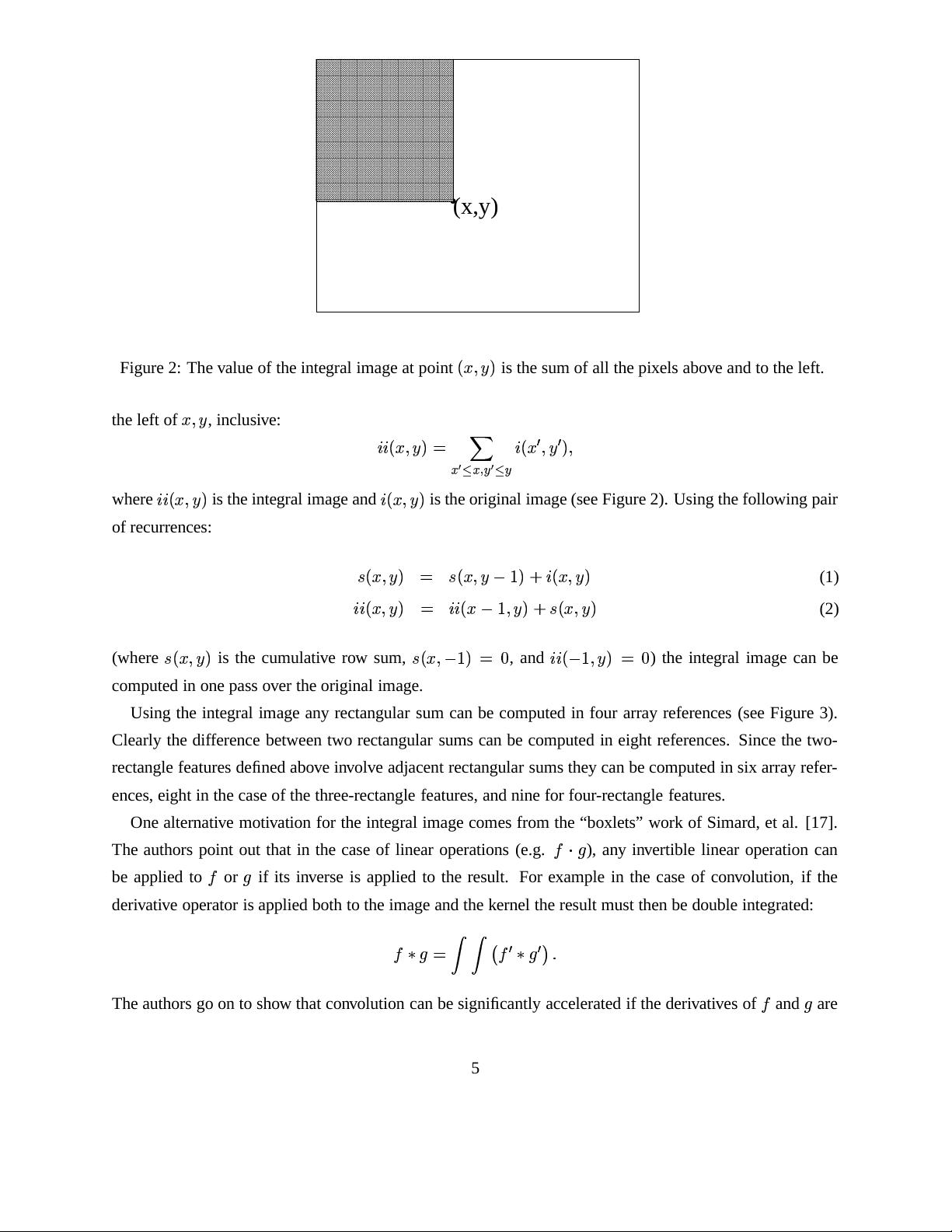
Figure 2: The value of the integral image at point
is the sum of all the pixels above and to the left.
the left of
, inclusive:
where
is the integral image and
is the original image (see Figure 2). Using the following pair
of recurrences:
(1)
!
"
#
(2)
(where
is the cumulative row sum,
$%&('
, and
%
)('
) the integral image can be
computed in one pass over the original image.
Using the integral image any rectangular sum can be computed in four array references (see Figure 3).
Clearly the difference between two rectangular sums can be computed in eight references. Since the two-
rectangle features defined above involve adjacent rectangular sums they can be computed in six array refer-
ences, eight in the case of the three-rectangle features, and nine for four-rectangle features.
One alternative motivation for the integral image comes from the “boxlets” work of Simard, et al. [17].
The authors point out that in the case of linear operations (e.g.
*,+-
), any invertible linear operation can
be applied to
*
or
-
if its inverse is applied to the result. For example in the case of convolution, if the
derivative operator is applied both to the image and the kernel the result must then be double integrated:
*)./-
102043
*
./-
6587
The authors go on to show that convolution can be significantly accelerated if the derivatives of
*
and
-
are
5


