[β
i1
, ⋯, β
in
]
T
is the output weight vector connecting the ith hidden
node and the output nodes.
The N equations can be rewritten compactly as:
Hβ ¼ Y ð2Þ
where
H ¼
h x
1
ðÞ
⋮
h x
N
ðÞ
2
4
3
5
¼
G ω
1
x
1
þ b
1
ðÞ⋯ G ω
L
x
1
þ b
L
ðÞ
⋮⋯⋮
G ω
1
x
N
þ b
1
ðÞ⋯ G ω
L
x
N
þ b
L
ðÞ
2
4
3
5
NL
ð3Þ
β ¼
β
T
1
⋮
β
T
L
2
4
3
5
Ln
and Y ¼
y
T
1
⋮
y
T
N
2
4
3
5
Nn
ð4Þ
H is called the hidden layer output matrix; the ith column of H is the
ith hidden node output with respect to inputs x
1
, x
2
, … , x
N
,theith row
of H is the hidden layer feature mapping with respect to the ith input x
i
.
β and Y represent the output weight matrix and output matrix,
respectively.
In general, the output weight matrix β is solved by minimizing the
approximation error in the squared error sense:
min
β∈R
Ln
Hβ−Ykk
F
ð5Þ
The optimal solution to Eq. (5) is given by
^
β ¼ H
þ
Y ð6Þ
where H
+
is the Moore–Penrose generalized inverse of the matrix H.
2.3. Proposed stacked ensemble ELM
Stacked generalization is a widely used and effective ensemble tech-
nique to combine (usually linearly) several different prediction sub-
models to improve predictive performance. In stacked generalization,
some ver sion of cross validation of sub-models is performed and the
predictions of sub-models during cross validation are stacked (denoted
as stacked X). The corresponding reference values of y are also stacked
(denoted as stacked y). A regression between stacked X and y can be
performed to determine the optimal weighted combination of predic-
tions from a library of candidate sub-models. Optimality is defined by
a user-specified objective function, such as minimizing the root mean
squared error of cross-validation (RMSECV) for the obtained final
model.
The proposed stacked ensemble ELM (SE-ELM) is very simple and
actually an application of ELM in the frame of stacked generalization.
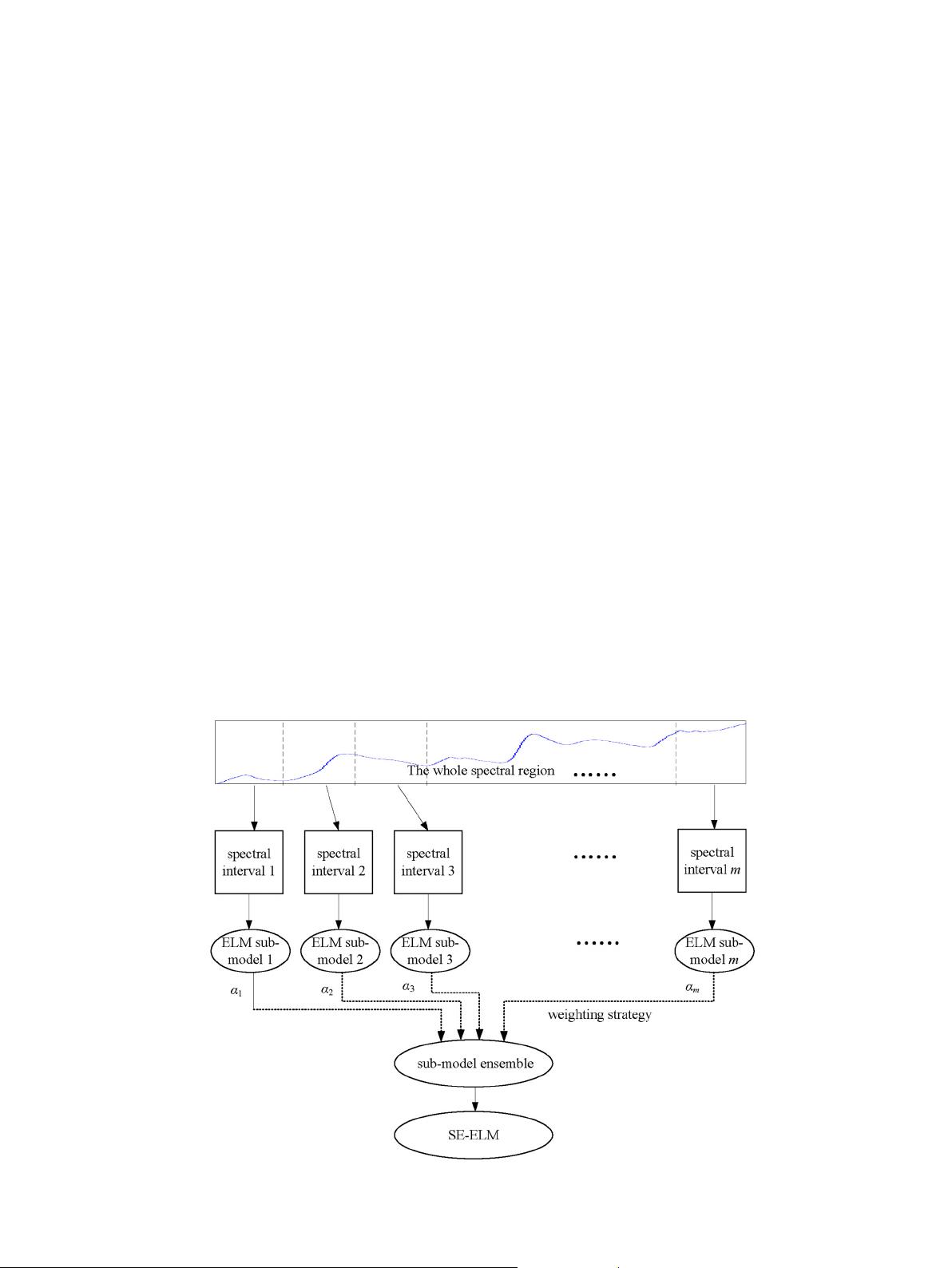
Fig. 2 shows the basic framework of SE-ELM model. The SE-ELM consists
of two key stages: sub-model generation and sub-model combination.
When SE-ELM is in the stage of sub-models generation, spectral interval
division is the key [31,32]. Firstly, original spectral matrix X is firstly
split into m disjoint intervals X
k
(k =1,2,… , m) of equal width (of p/
m variables). Then ELM based sub-models are generated to mine the
nonlinear relationship between each of the m intervals X
k
(k =1,2,…
,m) and the target property vector y. The number of intervals m can
be seen as a parameter to generate many sub-models. That is, the sub-
models are generated from the whole training set sampling from a pa-
rameter space. At the end of the entire cross-validation process of
each ELM sub-model, m different Monte Carlo cross-validated predicted
outputs
^
y
ELM‐MCCV
i
ði ¼ 1; ⋯; mÞ is obtained and then assembled to form a
matrix F ¼
^
y
ELM‐MCCV
1
;
^
y
ELM‐MCCV
2
; ⋯;
^
y
ELM‐MCCV
m
hi
. It is worth noting
that SE-ELM uses different number of hidden notes for all sub-interval
models. Namely, sub-interval models from different spectral region
have a different model complexity.
Once a collection of appropriate ELM based sub-models are gener-
ated from the whole calibration set, the subsequent step is to combine
these sub-models into an integrated model in an appropriate weighting
strategy. Generally, weighting strategi es include two kinds, linear
weighting methods and nonlinear weighting methods, in which the for-
mer are simple and most favored by users. Given this, we choose linear
Fig. 2. The basic framework of SE-ELM model.
99P. Shan et al. / Spectrochimica Acta Part A: Molecular and Biomolecular Spectroscopy 215 (2019) 97–111


