基于Pixel Recurrent Neural Networks的图像生成网络

需积分: 31 69 浏览量更新于2024-09-09 收藏 2.88MB PDF 举报

PRNN生成网络概述：PRNN（Pixel Recurrent Neural Networks）是一种深度学习生成网络，旨在解决自然图像的分布建模问题。该网络通过顺序预测图像中的像素值，捕捉图像中的所有依赖关系，实现图像生成和重构。 **生成网络** 生成网络是一种深度学习模型，旨在学习和生成自然图像的分布。PRNN生成网络通过递归神经网络（Recurrent Neural Networks，RNN）架构来实现图像生成，捕捉图像中的空间和时间依赖关系。 **Pixel Recurrent Neural Networks** PRNN生成网络的核心是Pixel Recurrent Neural Networks（Pixel RNN），它是一种递归神经网络架构，用于顺序预测图像中的像素值。该网络通过两种方式捕捉图像中的依赖关系：一是通过递归神经网络捕捉图像中的时间依赖关系，二是通过残差连接（Residual Connections）捕捉图像中的空间依赖关系。 **Fast Two-Dimensional Recurrent Layers** PRNN生成网络引入了快速的二维递归层（Fast Two-Dimensional Recurrent Layers），该层可以快速地捕捉图像中的空间依赖关系，提高了网络的训练速度和生成质量。 **Effective Use of Residual Connections** PRNN生成网络还引入了残差连接（Residual Connections），该技术可以有效地捕捉图像中的空间依赖关系，提高了网络的表达能力和生成质量。 **Log-Likelihood Scores** PRNN生成网络可以生成高质量的图像，同时也可以计算图像的似然分数（Log-Likelihood Scores），该分数可以评估生成图像的质量和真实性。 **Image Generation** PRNN生成网络可以生成高质量的图像，图像生成结果显示出很高的清晰度、多样性和全球一致性。 **Benchmark on ImageNet Dataset** PRNN生成网络在ImageNet数据集上的实验结果显示，该网络可以生成高质量的图像，超过了之前的状态-of-the-art结果。 **Conclusion** PRNN生成网络是一种强大的深度学习生成网络，能够生成高质量的自然图像，捕捉图像中的所有依赖关系。该网络的架构创新和技术创新为图像生成和重构提供了新的可能性。

Pixel Recurrent Neural Networks

The value p(x

, ..., x

i−1

) is the probability of the i-th

pixel x

given all the previous pixels x

, ..., x

i−1

. The gen-

eration proceeds row by row and pixel by pixel. Figure 2

(Left) illustrates the conditioning scheme.

Each pixel x

is in turn jointly determined by three values,

one for each of the color channels Red, Green and Blue

(RGB). We rewrite the distribution p(x

) as the fol-

lowing product:

p(x

i,R

)p(x

i,G

, x

i,R

)p(x

i,B

, x

i,R

, x

i,G

) (2)

Each of the colors is thus conditioned on the other channels

as well as on all the previously generated pixels.

Note that during training and evaluation the distributions

over the pixel values are computed in parallel, while the

generation of an image is sequential.

2.2. Pixels as Discrete Variables

Previous approaches use a continuous distribution for the

values of the pixels in the image (e.g. Theis & Bethge

(2015); Uria et al. (2014)). By contrast we model p(x) as

a discrete distribution, with every conditional distribution

in Equation 2 being a multinomial that is modeled with a

softmax layer. Each channel variable x

i,∗

simply takes one

of 256 distinct values. The discrete distribution is represen-

tationally simple and has the advantage of being arbitrarily

multimodal without prior on the shape (see Fig. 6). Exper-

imentally we also ﬁnd the discrete distribution to be easy

to learn and to produce better performance compared to a

continuous distribution (Section 5).

3. Pixel Recurrent Neural Networks

In this section we describe the architectural components

that compose the PixelRNN. In Sections 3.1 and 3.2, we

describe the two types of LSTM layers that use convolu-

tions to compute at once the states along one of the spatial

dimensions. In Section 3.3 we describe how to incorporate

residual connections to improve the training of a PixelRNN

with many LSTM layers. In Section 3.4 we describe the

softmax layer that computes the discrete joint distribution

of the colors and the masking technique that ensures the

proper conditioning scheme. In Section 3.5 we describe the

PixelCNN architecture. Finally in Section 3.6 we describe

the multi-scale architecture.

3.1. Row LSTM

The Row LSTM is a unidirectional layer that processes

the image row by row from top to bottom computing fea-

tures for a whole row at once; the computation is per-

formed with a one-dimensional convolution. For a pixel

the layer captures a roughly triangular context above the

pixel as shown in Figure 4 (center). The kernel of the one-

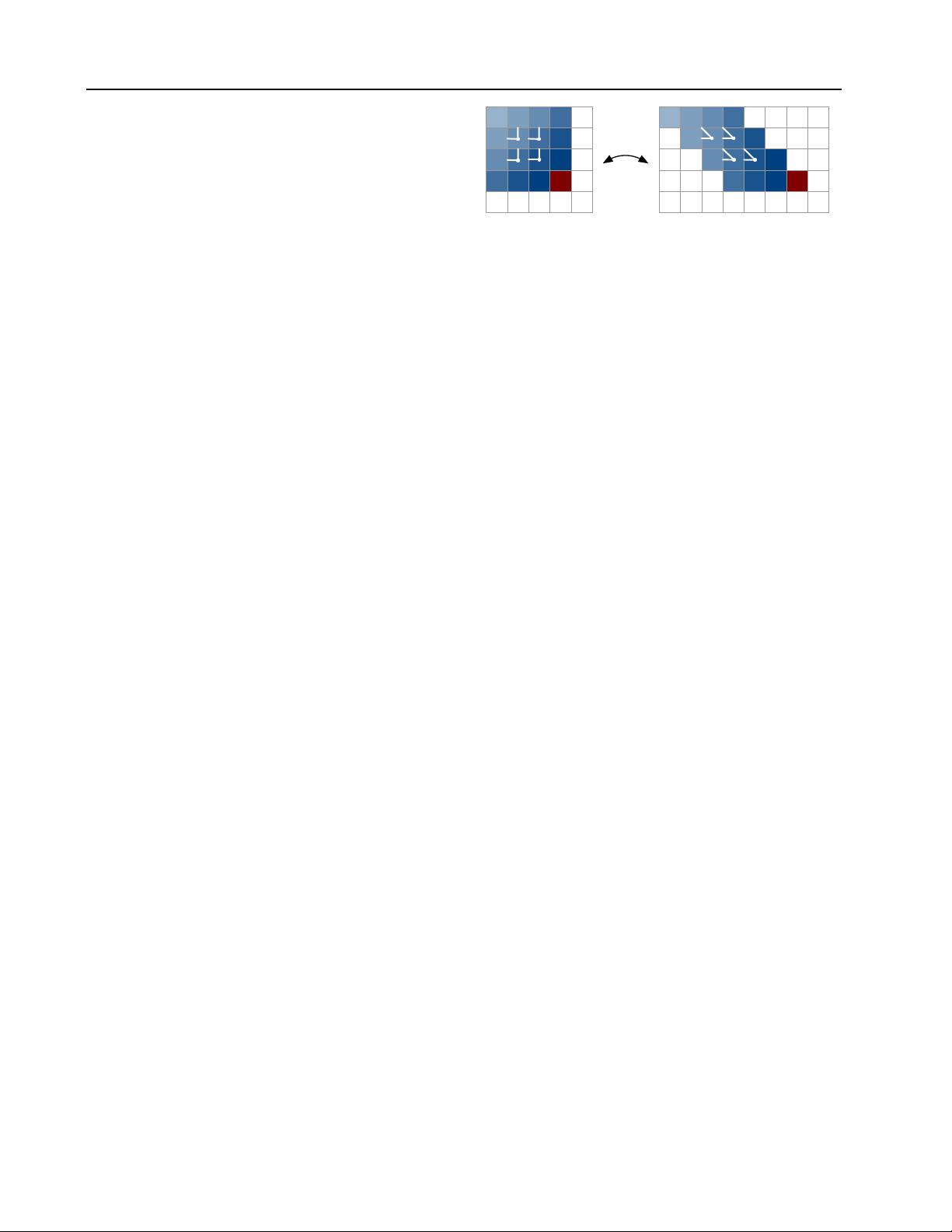
Figure 3. In the Diagonal BiLSTM, to allow for parallelization

along the diagonals, the input map is skewed by offseting each

row by one position with respect to the previous row. When the

spatial layer is computed left to right and column by column, the

output map is shifted back into the original size. The convolution

uses a kernel of size 2 × 1.

dimensional convolution has size k × 1 where k ≥ 3; the

larger the value of k the broader the context that is captured.

The weight sharing in the convolution ensures translation

invariance of the computed features along each row.

The computation proceeds as follows. An LSTM layer has

an input-to-state component and a recurrent state-to-state

component that together determine the four gates inside the

LSTM core. To enhance parallelization in the Row LSTM

the input-to-state component is ﬁrst computed for the entire

two-dimensional input map; for this a k × 1 convolution is

used to follow the row-wise orientation of the LSTM itself.

The convolution is masked to include only the valid context

(see Section 3.4) and produces a tensor of size 4h × n × n,

representing the four gate vectors for each position in the

input map, where h is the number of output feature maps.

To compute one step of the state-to-state component of

the LSTM layer, one is given the previous hidden and cell

states h

i−1

and c

i−1

, each of size h × n × 1. The new

hidden and cell states h

, c

are obtained as follows:

, f

, i

, g

] = σ(K

~ h

i−1

+ K

~ x

)

= f

 c

i−1

+ i

 g

= o

 tanh(c

)

(3)

where x

of size h × n × 1 is row i of the input map, and

~ represents the convolution operation and  the element-

wise multiplication. The weights K

and K

are the

kernel weights for the state-to-state and the input-to-state

components, where the latter is precomputed as described

above. In the case of the output, forget and input gates o

and i

, the activation σ is the logistic sigmoid function,

whereas for the content gate g

, σ is the tanh function.

Each step computes at once the new state for an entire row

of the input map. Because the Row LSTM has a triangular

receptive ﬁeld (Figure 4), it is unable to capture the entire

available context.

剩余10页未读，继续阅读

weixin_44276261

粉丝: 1
资源: 49

基于Pixel Recurrent Neural Networks的图像生成网络

matlab的egde源代码-3D-PRNN:火炬实施我们的ICCV17论文：“3D-PRNN，使用递归神经网络生成形状基元”

bmp显示，旋转及prn转化

prn格式文件打印工具

matlabalexnet图像识别代码-PRNNFinalProject:PRNN最终项目

RNNWavefunctions:基于递归神经网络的波函数ansatz进行变分蒙特卡罗模拟

VB程序实例-运用Mschat图表显示数据(方法二).zip

VB程序实例-改变Windows图标大小.zip

技术资料分享ZigBee协议栈的研究与实现非常好的技术资料.zip

pytz-2016.10-py3.1.egg

技术资料分享ADV7123非常好的技术资料.zip

最新资源