风险资产估值与投资选择：Lintner理论解析

需积分: 10 142 浏览量更新于2024-07-15 收藏 859KB PDF 举报

《风险资产估值与投资组合选择》是约翰·林特纳（John Lintner）在1965年发表于《经济学与统计学评论》(The Review of Economics and Statistics)第47卷第1期的一篇文章，其研究焦点集中在金融市场中风险资产的价值评估以及投资者如何根据这些评估来挑选高风险投资。林特纳在这篇经典论文中提出了著名的套利定价理论(Arbitrage Pricing Theory, APT)，该理论为理解非均衡市场中的资产定价提供了全新的视角。在文中，林特纳探讨了如何在存在风险和不确定性的情况下，通过构建投资组合来分散风险，同时考虑预期收益和风险之间的关系。他强调了资本预算决策中的风险评估，特别是在股票投资组合管理中，投资者不仅要关注单个资产的回报，还要考虑资产间的相关性对整体风险的影响。林特纳的模型指出，投资者可以通过多元化的投资策略，即构建一个包含不同风险等级和收益预期的资产组合，来实现最优的风险调整后收益，也就是著名的夏普比率(Sharpe Ratio)。他提出的理论认为，资产的价格应该反映其风险溢价，即投资者为了承担额外风险而要求的补偿，这是资产定价的一个关键因素。这一理论有助于金融机构、企业和个人投资者在复杂的金融环境中做出更为理性的投资决策，避免仅仅基于期望收益率进行投资，而是要综合考虑风险和回报的平衡。林特纳的工作对现代金融学有着深远的影响，不仅深化了我们对风险的理解，而且为现代投资组合理论奠定了基础。通过对风险资产的估值和投资选择的研究，投资者可以更有效地管理他们的投资组合，提高投资效率，并在面对不确定性和波动性时做出更明智的选择。文章的发表标志着对资产定价理论的重要突破，它为后续的金融工程和实证研究提供了理论支持，同时也推动了金融市场的实践发展，比如在资产定价模型、期权定价和风险管理等领域。这是一篇在投资理论和实践中具有里程碑意义的研究成果，对于理解金融市场、优化投资组合以及风险管理具有不可替代的价值。

THE

REVIEW

ECONOMICS

AND

STATISTICS

With

respect

to an

investor's criterion

for

choices among different attainable combinations

of assets, we assume that (3) if any two mixtures

of assets have the same expected return, the inves-

tor

will

prefer

the one

having the

smaller

variance

of return, and

any two mixtures of assets have

the same variance

returns,

he will

prefer the

one having

the

greater expected

value. Tobin

[21,

pp.

75-761 has shown that such preferences are

implied by maximization of the expected value

a von

Neumann-Morgenstern utility

function

if either

(a)

the

investor's utility function is con-

cave and

quadratic

(b)

the

investor's utility

function is

concave,

and he

has assigned probabil-

ity distributions such that the returns on

all

pos-

sible

portfolios differ

most

location

and

scale

parameter, (which

will

the

case

the joint

dis-

tribution

all individual stocks is multivariate

normal).

Alternative Proofs of

the

Separation

Theorem

Since

the interest rates on

riskless

savings

bank

deposits ("loans

to the

bank")

and

bor-

rowed funds are being assumed to be the

same,

we can treat borrowing as negative lending.

Any portfolio

can

then

be described

terms of

(i)

the

gross

amount invested in

stocks, (ii) the

fraction of this amount invested

each indivi-

dual

stock,

and

(iii)

the

net

amount invested in

loans (a negative

value

showing

that the investor

has

borrowed rather than

lent).

But since

the

total net

investment

(the algebraic

sum of

stocks

plus loans)

is a

given arnount,

the

problem

sim-

ply requires finding the jointly optimal values

for

(1)

the ratio of the

gross

investment

stocks

the total net

investment,

and

(2)

the ratio of

the

gross

investment

each individual stock

the

total

gross

investment

stocks.

It turns out

that

although

the solution of

(1) depends upon

that

(2),

our

context the latter is

indepen-

dent

the former.

Specifically,

the

separation

theorem

asserts

that:

Given the

assumptions

about

borrowing,

lending,

and

investor

preferences stated earlier

this

section,

the

optimal proportionate composition

the

stock

(risk-asset) portfolio (i.e.

the solution

sub-problem

above)

independent of

the

ratio

the

gross

investment

stocks

the total

net

investment.

Tobin

proved

this

important separation theo-

ren by deriving

the detailed solution for

the

optimal

mix

of risk assets conditional on

given

gross

investment

this

portfolio,

and then

for-

mally

proving

the

critical

invariance

property

stated

in the theorem.

Tobin

used more

restric-

tive

assumnptions

that we

regarding

the

avail-

able

investment

opportunities

and he

pernmitted

borrowing."

Under

our

somewhat broadened

assumptions

these

respects,

the

problem

fits

neatly into a traditional Fisher

framework,

with

different

available

combinations

expected

values

and

standard deviations of return on

al-

ternative stock

portfolios

taking

the

place

the

original "production

opportunity"

set and

with. the

alternative investment

choices

being

concurrent rather than

between time

periods.

Within

this

frarmework,

alternative and

transparent

proofs

the

separation theorem

are available which do not

involve the

actual

calculation

the best allocation in

stocks

over

individual

stock

issues. As did

Fisher, we shall

present a

simple

algebraic proof

12, set

out the

logic

the

argument

lea-ding

to the

theorem, and

depict

the

essential

geomretry

the

problemr.13

As a

preliminary step, we need

establish

the

relation between

the

investor's

total

investment

any

arbitrary

mixture

or portfolio

individual

stocks,

his

total net return from

all

his invest-

nments

(including risliless assets

and any borrow-

ing), and

the

risk

parameters of

his

investment

position.

Let the interest rate on

riskless

assets

borrowing

r*,

and the

uncertain

return

(divi-

dends

plus price

appreciation) per dollar

invested

the

given

portfolio of

stocks be

r. Let w

rep-

resent

the ratio

of gross

investment in

stocks to

"1Tobin

considered

the

special

case where

cash

with

return

was the

only

riskless

asset available.

While

formally

required that

all

assets be

held

non-negative

quantities

(thereby

ruling out

short

sales), and

that the

total value of risk

assets

held

not be

greater

than

the

investment

balance

available

without

borrowing,

these

non-negativity

and

maximum

value

constraints

were

not

introduced

into his formal

solution

the

optimal

investment mix,

which

turn

was used in

proving

the

invariance

property

stated in

the

theorem.

Our

proof of

the

theorem is

independent

the

programming

constraints

neglec-

ted

Tobin's

proof. Later

this

section we show

that

when

short sales are

properly and

explicitly

introduced

into

the set

possible

portfolios, the

resulting

equations for

the

optimum

portfolio mix are

identical to

those

derived

Tobin,

but

that

insistence on

short

sales

results

somewhat

complex

programming

problem

(when

covariances

are

non-zero),

which

may

however,

readily

handled

with

computer

programs

now

available.

12An

alternative

algebraic proof

using

utility

functions

explicitly is

presented

the

appendix,

note I.

Lockwood

Rainhard, Jr.

has

also

independently

developed

and

presented a

similar

proof

of the

theorem in

unpublished

seminar

paper.

This content downloaded from 192.231.202.205 on Thu, 4 Dec 2014 14:48:30 PM

All use subject to JSTOR Terms and Conditions

VALUATION OF RISK ASSETS

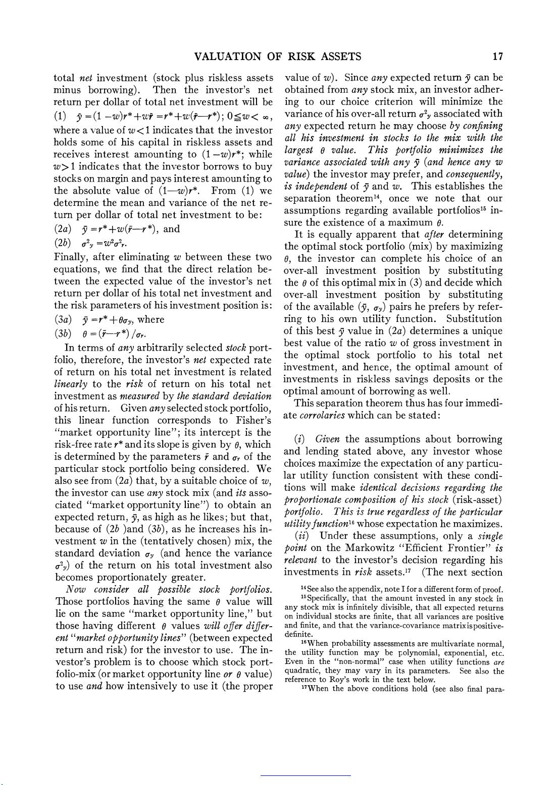
total net investment

(stock plus

riskless

assets

minus borrowing).

Then the investor's net

return per dollar of

total net investment will be

(1)

=(1 -w)r*+wf

=r*+w(f-r*); O?<w< o,

where

alue of w <

indicates

that the

investor

holds

some

of his

capital

riskless

assets

and

receives interest

amounting to (1 -w)r*; while

indicates that

the investor borrows to buy

stocks on margin and

pays

interest

amounting

the

absolute value

(1-w)r*. From (1) we

determine

the

mean and variance

the net re-

turn

per

dollar of total

net investment to be:

(2a) y

=r*+w(-r*),

and

(2b) a2y=W2.,2r.

Finally, after

eliminating

between these

two

equations,

we find

that

the

direct relation be-

tween

the

expected value

the

investor's net

return per dollar of

his total net

investmnent

and

the

risk

parameters

of his

investment

position

is:

(3a) y

=r*

+Ouy,

where

(3b)

(r-S

*) /0ru

terms of any

arbitrarily selected stock port-

folio, therefore,

the investor's

net

expected rate

return

his total net investment is

linearly

to the

risk

return on his

total

net

investment as

measured

the standard

deviation

of his

return. Given

any

selected stock

portfolio,

this linear function

corresponds

Fisher's

"market

opportunity line";

its

intercept

the

risk-free rate r* and its

slope

given by 0, which

determined

the

parameters r

and

u,.

the

particular

stock

portfolio

being

considered.

also

see

from

(2a)

that, by

suitable choice

the

investor

can use

any

stock

mix

(and

its asso-

ciated "market

opportunity line")

to obtain an

expected return, y,

high

likes;

but

that,

because

(2b )and

(3b),

as he

increases his in-

vestment

w in

the

(tentatively chosen) mix, the

standard deviation

(and

hence

the

variance

a2y)

the

return on his

total

investment also

becomes

proportionately greater.

Now

consider

all

possible

stock

portfolios.

Those portfolios

having

the same

0 value will

lie

the same

"market opportunity line," but

those

having

different

values will

ojjer

dijTer-

ent "market

opportunity

lines"

(between expected

return and

risk)

for

the

investor

use. The

in-

vestor's

problem

to choose

which stock

port-

folio-mix

(or

market

opportunity

line

value)

to use and how

intensively

to use it

(the proper

value of w). Since any expected return y can

obtained from any stock

mix,

an investor

adher-

ing to our choice criterion will

minimize

the

variance of his over-all return

o2y

associated

with

any expected return he may choose by confining

all

his investment

in stocks

to the

mix

with

the

larges?

value.

This portfolio minimizes the

variance associated with

any

(and

hence

any

value)

the investor

may prefer,

and

consequently,

independent of y and w.

This establishes

the

separation theorem'4, once we note that our

assumptions regarding available portfolios'5

in-

sure the existence of a maximum 0.

It is equally apparent that after determining

the optimal stock portfolio (mix) by maximizing

the investor can

complete

his choice

over-all investment position by substituting

the

this optimal

mix in

(3)

and

decide

which

over-all investment position by substituting

the available (y,

ay)

pairs he prefers by refer-

ring to his own utility function. Substitution

this best y value in (2a) determines a unique

best value

the ratio

w of

gross investment

the

optimal

stock

portfolio

to his total net

investment, and hence, the optimal amount

investments in riskless savings deposits or the

optimal amount of borrowing as well.

This

separation theorem thus has four

immedi-

ate

corrolaries which can be

stated:

(i)

Given the

assumptions

about

borrowing

and

lending

stated

above, any

investor

whose

choices maximize the

expectation

any particu-

lar utility function consistent with these condi-

tions

will make

identical

decisions

regarding

the

proportionate composition of

his

stock (risk-asset)

portfolio.

This is

true regardless of the particular

utility functionl6

whose

expectation he maximizes.

(ii)

Under

these

assumptions, only a single

point

the

Markowitz "Efficient Frontier" is

relevant

the

investor's decision

regarding his

investments

risk assets.17 (The next section

14See also the

appendix,

note

for a

different form of

proof.

15Specifically,

that

the

amount

invested

any

stock in

any

stock mix

infinitely

divisible,

that

all

expected

returns

individual

stocks are

finite,

that

all

variances

are

positive

and

finite,

and

that the

variance-covariance

matrixispositive-

definite.

16When

probability

assessments

are

multivariate

normal,

the

utility

function

may

polynomial,

exponential,

etc.

Even

the "non-normal"

case

when

utility

functions

are

quadratic,

they

may

vary

its

parameters. See

also

the

reference to

Roy's

work

the

text

below.

17When

the

above

conditions

hold

(see

also

final

para-

This content downloaded from 192.231.202.205 on Thu, 4 Dec 2014 14:48:30 PM

All use subject to JSTOR Terms and Conditions

剩余25页未读，继续阅读

Quant0xff

粉丝: 1w+
资源: 459

风险资产估值与投资选择：Lintner理论解析

"国际私募股权和风险投资估值指引（2018版）英文版详解

"资本资产定价模型及其应用——第7章节概述

"高盛：墨西哥股票与债券错位投资策略的新兴市场趋势

John.Wiley.&.Sons.-.Investment.Valuation.-.Tools.&.Techniques.for.Determining.the.Value.of.Any.Asset.2ed.[2002]

CFA 一级试题 十五 Asset Valuation Debt Investments Analysis and Valuation_removed.pdf

CFA 一级试题 十六 Asset Valuation Derivative Investments_removed.pdf

CFA 一级试题 十七 Asset Valuation Alternative Investments_removed.pdf

CFA 一级试题 十三 Asset Valuation Equity Investments_removed.pdf

债券估值的Excel操作Bond-Valuation.pdf

Chapter 8 Valuation of Bonds(Finance -东北财经大学).pdf

最新资源

CFA 一级试题十五 Asset Valuation Debt Investments Analysis and Valuation_removed.pdf

CFA 一级试题十六 Asset Valuation Derivative Investments_removed.pdf

CFA 一级试题十七 Asset Valuation Alternative Investments_removed.pdf

CFA 一级试题十三 Asset Valuation Equity Investments_removed.pdf