没有合适的资源?快使用搜索试试~ 我知道了~
首页关于OFDM通信系统中信道估计的综述报告
关于OFDM通信系统中信道估计的综述报告
4星 · 超过85%的资源 需积分: 9 21 下载量 129 浏览量
更新于2023-07-14
3
收藏 638KB PDF 举报
本文是关于OFDM通信系统中信道估计的综述报告,讲解十分全面,看完本文可以了解近年来信道估计发展的方向和水平
资源详情
资源推荐
IEEE Communications Surveys & Tutorials • 2nd Quarter 2007
18
riven by multimedia based applications, anticipated
future wireless systems will require high data rate
capable technologies. Novel techniques such as
OFDM and MIMO stand as promising choices for future high
data rate systems [1, 2].
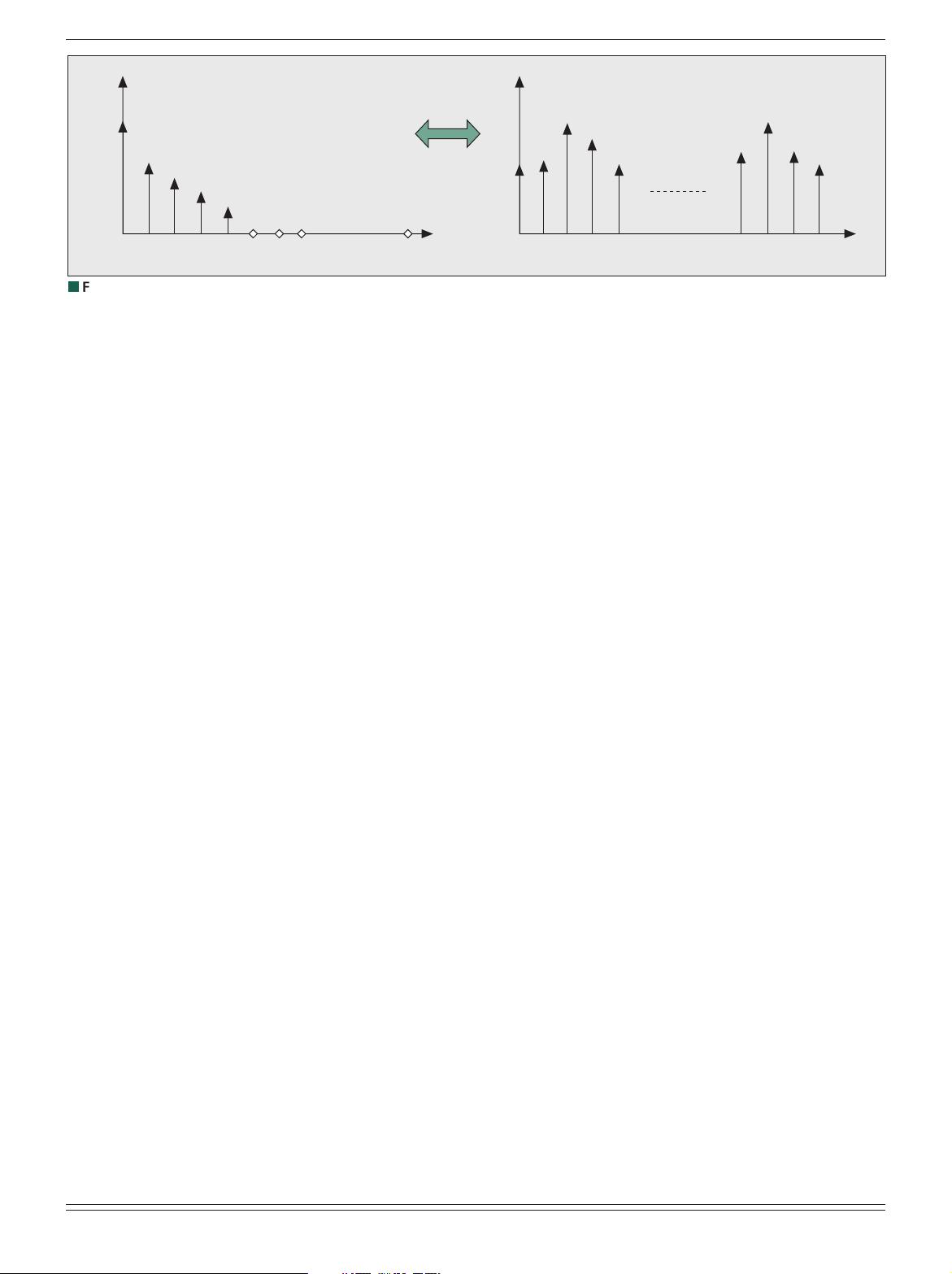
OFDM divides the available spectrum into a number of
overlapping but orthogonal narrowband subchannels, and
hence converts a frequency selective channel into a non-
frequency selective channel [3]. Moreover, ISI is avoided by
the use of CP, which is achieved by extending an OFDM
symbol with some portion of its head or tail [4]. With these
vital advantages, OFDM has been adopted by many wire-
less standards such as DAB, DVB, WLAN, and WMAN [5,
6].
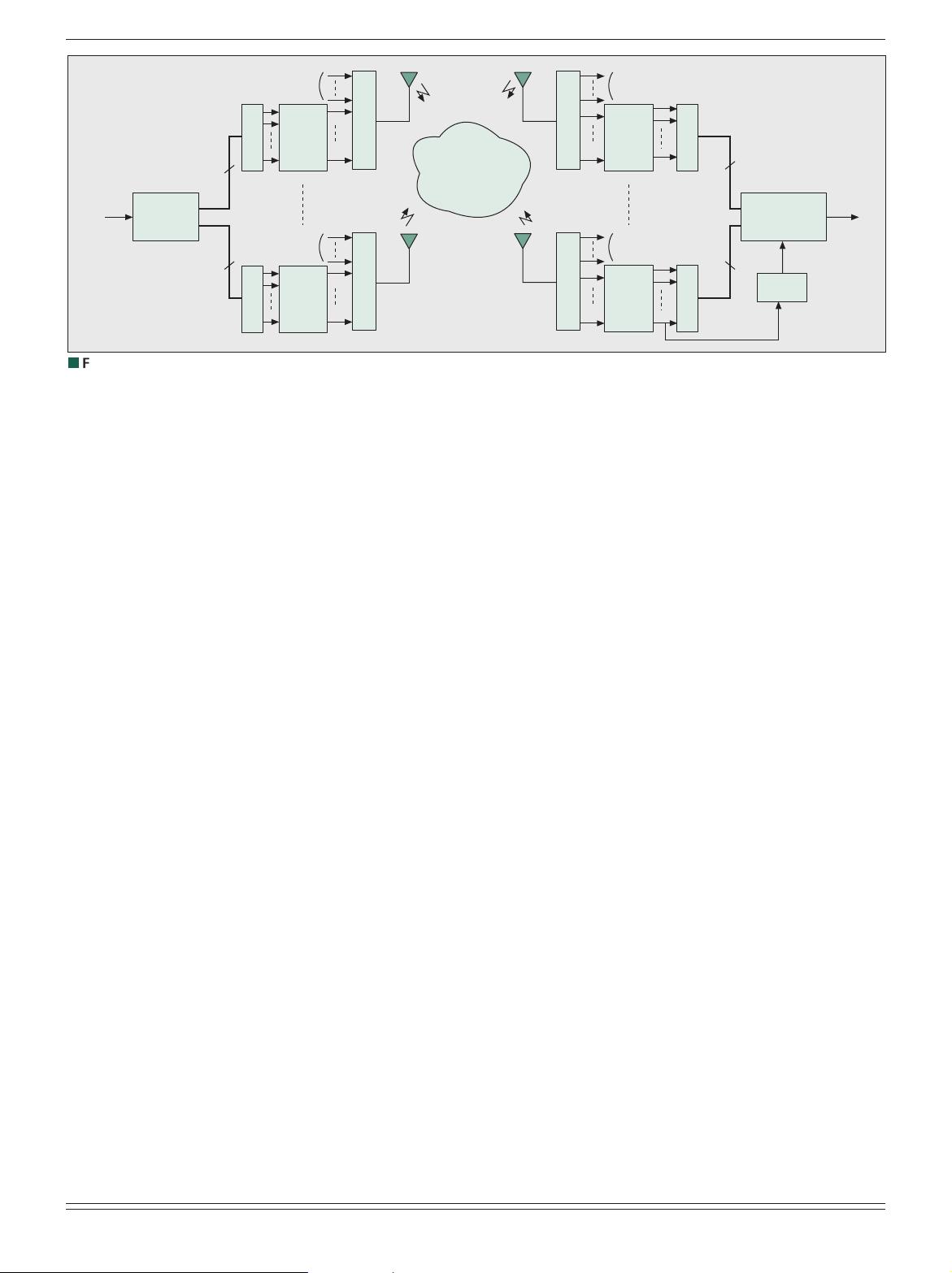
MIMO, on the other hand, employs multiple antennas at
the transmitter and receiver sides to open up additional sub-
channels in spatial domain. Since parallel channels are estab-
lished over the same time and frequency, high data rates
without the need of extra bandwidth are achieved [7, 8]. Due
to this bandwidth efficiency, MIMO is included in the stan-
dards of future BWA [9]. Overall, these benefits have made
the combination of MIMO-OFDM an attractive technique for
future high data rate systems [10–12].
As in many other coherent digital wireless receivers, chan-
nel estimation is also an integral part of the receiver designs
in coherent MIMO-OFDM systems [13]. In wireless systems,
transmitted information reaches to receivers after passing
through a radio channel. For conventional coherent receivers,
the effect of the channel on the transmitted signal must be
estimated to recover the transmitted information [14]. As long
as the receiver accurately estimates how the channel modifies
the transmitted signal, it can recover the transmitted informa-
tion. Channel estimation can be avoided by using differential
modulation techniques, however, such systems result in low
data rate and there is a penalty for 3–4 dB SNR [15 19]. In
some cases, channel estimation at user side can be avoided if
the base station performs the channel estimation and sends a
pre-distorted signal [20]. However, for fast varying channels,
the pre-distorted signal might not bear the current channel
distortion, causing system degradation. Hence, systems with a
channel estimation block are needed for the future high data
rate systems.
Channel estimation is a challenging problem in wireless
systems. Unlike other guided media, the radio channel is high-
ly dynamic. The transmitted signal travels to the receiver by
undergoing many detrimental effects that corrupt the signal
D
MEHMET KEMAL OZDEMIR, LOGUS BROADBAND WIRELESS SOLUTIONS, INC. AND
HUSEYIN ARSLAN, UNIVERSITY OF SOUTH FLORIDA
ABSTRACT
Orthogonal frequency division multiplexing (OFDM) is a special case of
multi-carrier transmission and it can accommodate high data rate require-
ment of multimedia based wireless systems. Since channel estimation is an
integral part of OFDM systems, it is critical to understand the basis of
channel estimation techniques for OFDM systems so that the most appro-
priate method can be applied. In this article, an extensive overview of chan-
nel estimation techniques employed in OFDM systems are presented. In
addition, the advantages, drawbacks, and relationship of these estimation
techniques with each other are analyzed and discussed. As the combination
of multiple input multiple output (MIMO)-OFDM systems promises higher
data rates, estimation techniques are further investigated for these systems.
Although the existing proposed techniques differ in terms of computational
complexity and their mean squared error (MSE) performance, it has been
observed that many channel estimation techniques are indeed a subset of
LMMSE channel estimation technique. Hence, based on a given system’s
resources and specifications, a suitable method among the presented tech-
niques can be applied.
CHANNEL ESTIMATION FOR
WIRELESS OFDM SYSTEMS
2ND QUARTER 2007, VOLUME 9, NO. 2
www.comsoc.org/pubs/surveys
1553-877X
IEEE Communications Surveys & Tutorials • 2nd Quarter 2007
19
and often place limitations on the performance of the system.
Transmitted signals are typically reflected and scattered, arriv-
ing at receivers along multiple paths. Also, due to the mobility
of transmitters, receivers, or scattering objects, the channel
response can change rapidly over time. Most important of all,
the radio channel is highly random and the statistical charac-
teristics of the channel are environment dependent. Multipath
propagation, mobility, and local scattering cause the signal to
be spread in frequency, time, and angle. These spreads, which
are related to the selectivity of the channel, have significant
implications on the received signal. Channel estimation per-
formance is directly related to these statistics. Different tech-
niques are proposed to exploit these statistics for better
channel estimates. There has been some studies that cover
these estimation techniques, however these are limited to the
comparison of few of the channel estimation techniques
[21–24]. This paper focuses on an extensive overview of the
channel estimation techniques commonly applied to OFDM
based multi-carrier wireless systems.
OFDM CHANNEL ESTIMATION
Channel estimation has a long and rich history in single carri-
er communication systems. In these systems, the CIR is typi-
cally modeled as an unknown time-varying FIR filter, whose
coefficients need to be estimated [14]. Many of the channel
estimation approaches of single carrier systems can be applied
to multi-carrier systems. However, the unique properties of
multi-carrier transmission bring about additional perspectives
that allow the development of new approaches for channel
estimation of multi-carrier systems.
In OFDM based systems, the data is modulated onto the
orthogonal frequency carriers. For coherent detection of the
transmitted data, these sub-channel frequency responses must
be estimated and removed from the frequency samples. Like
in single carrier systems, the time domain channel can be
modelled as a FIR filter, where the delays and coefficients can
be estimated from time domain received samples, which are
then transformed to frequency domain for obtaining the CFR.
Alternatively, radio channel can also be estimated in frequen-
cy domain using the known (or detected) data on frequency
domain sub-channels. Instead of estimating FIR coefficients,
one tap CFR can be estimated (Fig. 1).
Channel estimation techniques for OFDM based systems
can be grouped into two main categories: blind and non-blind.
The blind channel estimation methods exploit the statistical
behavior of the received signals and require a large amount of
data [25]. Hence, they suffer severe performance degradation
in fast fading channels [26]. On the other hand, in the non-
blind channel estimation methods, information of previous
channel estimates or some portion of the transmitted signal
are available to the receiver to be used for the channel esti-
mation. In this article, only the non-blind channel estimation
techniques will be investigated.
The non-blind channel estimation can be studied under
two main groups: data aided and DDCE. In data aided chan-
nel estimation, a complete OFDM symbol or a portion of a
symbol, which is known by the receiver, is transmitted so that
the receiver can easily estimate the radio channel by demodu-
lating the received samples. Often, frequency domain pilots
are employed similar to those in new generation WLAN stan-
dards (802.11a and HYPERLAN2) [27]. The estimation accu-
racy can be improved by increasing the pilot density. However,
this introduces overhead and reduces the spectral efficiency.
In the limiting case, when pilot tones are assigned to all sub-
carriers of a particular OFDM symbol, an OFDM training
symbol can be obtained (block type pilot arrangement). This
type of pilot arrangement is usually considered for slow chan-
nel variation and for burst type data transmission schemes,
where the channel is assumed to be constant over the burst.
The training symbols are then inserted at the beginning of the
bursts to estimate the CFR (e.g. WLAN and WiMAX sys-
tems) [28, 29]. When channel varies between consecutive
OFDM symbols, either the training symbols should be insert-
ed regularly within OFDM data symbols with respect to the
time variation of the channel (Doppler spread), or the chan-
nel should be tracked in a decision directed mode to enhance
the receiver performance.
In the DDCE methods, to decode the current OFDM sym-
bol the channel estimates for a previous OFDM symbol are
used. The channel corresponding to the current symbol is
then estimated by using the newly estimated symbol informa-
tion. Since an outdated channel is used in the decoding pro-
cess, these estimates are less reliable as the channel can vary
drastically from symbol to symbol [31, 32]. Hence, additional
information is usually incorporated in DDCE such as periodi-
cally sent training symbols. Channel coding, interleaving, and
iterative type approaches are also commonly applied to boost
the performance of DDCE~techniques.
There are numerous approaches to estimate the channels
for OFDM subcarriers. The direct estimation of the channel
for subcarriers treats each subcarrier as if the channels are
independent. However, in practice, the CFR is often oversam-
pled via the subcarriers, and hence the estimated frequency
domain channel coefficients are correlated. On the other
hand, the noise in these subcarriers can be independent. By
utilizing the correlation of CFR in subcarriers, the noise can
be reduced significantly. Therefore, the channel estimation
accuracy can be improved [28]. Several approaches have been
proposed to exploit this correlation. These approaches and
their relationship with each other will be discussed in the sub-
sequent sections to provide a unified understanding. Similarly,
the subcarrier correlation in time and spatial domain can be
exploited since the noise can be considered to be independent
in time and spatial domain as well.
n
Figure 1. Time and frequency domain channels representation for OFDM based systems.
Tap index
CIR
CFR
Coefficients
Coefficients
DFT/IDFT
Subcarrier index
IEEE Communications Surveys & Tutorials • 2nd Quarter 2007
20
Although it is a common approach to assume the channel
to be constant over an OFDM symbol duration [9, 27], for
fast fading channels the same assumption leads to ICI [33],
which degrades the channel estimation performance. Hence,
the methods employed in data-aided and decision directed
channel estimation need to be modified so that the variation
of the channel over the OFDM symbol is taken into account
for better estimates. External interfering sources also affect
the performance of channel estimation. The effect of interfer-
ing sources can be mitigated by exploiting their statistical
properties. Although most systems treat ICI and external
interference as part of noise, better channel estimation perfor-
mance can be obtained by more accurate modeling [34].
There are basically three basic blocks affecting the perfor-
mance of the non-blind channel estimation techniques. These
are the pilot patterns, the estimation method, and the signal
detection part. Each method covered in this article either
tackles one of the above basic block or several at a time. The
specific choice depends on the wireless system specifications
and the channel condition. The aspects of each method are
presented such that a suitable method can easily be selected
for a given wireless system and channel conditions. It can be
observed that each method can be approximated to the other
methods by using the same set of variables. For example, in
this paper it is shown that each estimation method is indeed a
subset of LMMSE technique.
In the literature, initial channel estimation methods have
been mostly developed for SISO-OFDM systems, that is, sin-
gle antenna systems. With the emergence of MIMO-OFDM,
these methods need some modifications as the received signal
in MIMO-OFDM is the superposition of all the transmitted
signals of a given user. In many cases, the methods of SISO-
OFDM are easily adopted for MIMO-OFDM but novel meth-
ods exploiting space-time codes or other MIMO specific
elements are also introduced.
In the rest of the article, starting from a generic system
model, the channel estimation techniques will be presented
starting from the less complicated techniques. More emphasis
will be given on data aided channel estimation as it provides
some unique approaches for OFDM systems. Discussions on
ICI, external interferers, and MIMO systems as well as related
issues will also be given. Finally, some concluding remarks and
potential research areas will be given at the end of the article.
NOTATION
Matrices and the vectors are denoted with boldface letters,
where the upper/lower letters will be used for frequency/time
domain variables; (.)
H
denotes conjugate-transpose; E{.}
denotes expected value; diag(x) stands for diagonal matrix
with the column vector x on its diagonal; 0
a×b
denotes a
matrix of a × b with zero entries; IN denotes N × N identity
matrix; and j=√
——
–1.
SYSTEM MODEL
A generic block diagram of a basic baseband-equivalent
MIMO-OFDM system is given in Fig. 2. A MIMO-OFDM
system with N
tx
transmit and N
rx
receive antennas is assumed.
The information bits can be coded and interleaved. The coded
bits are then mapped into data symbols depending on the
modulation type. Another stage of interleaving and coding
can be performed for the modulated symbols. Although the
symbols are in time domain, the data up to this point is con-
sidered to be in the frequency domain. The data is then de-
multiplexed for different transmitter antennas. The serial data
symbols are then converted to parallel blocks, and an IFFT is
applied to these parallel blocks to obtain the time domain
OFDM symbols. For the transmit antenna, tx, time domain
samples of an OFDM symbol can be obtained from frequency
domain symbols as
(1) (1)
(2)
where X
tx
[n, k] is the data at the kth subcarrier of the nth
OFDM symbol, K is the number of subcarriers, and m is the
time domain sampling index. After the addition of CP, which
is larger than the expected maximum excess delay of the chan-
nel, and D/A conversion, the signals from different transmit
antennas are sent through the radio channel.
The channel between each transmitter/receiver link is mod-
elled as a multi-tap channel with the same statistics [3]. The
typical channel at time t is expressed as,
(3)
where L is the number of taps, α
l
is the lth complex path gain,
and τ
l
is the corresponding path delay. The path gains are
WSS complex Gaussian processes. The individual paths can be
ht t
ll
l
L
(, ) () ( ),
ταδττ
= −
=
−
∑
0
1
x n m IFFT X n k
Xn
tx tx
tx
[, ] { [, ]}
[,
=
= kke km K
k
K
jmkK
],
/
=
−
∑
≤≤−
0
1
2
01
π
n
Figure 2. MIMO-OFDM transceiver model.
Wireless
channel
S
/
P
P
/
S
S
/
P
X
1
X
Ntx
K
K
Y
1
Y
Nrx
K
K
Ant #1 Ant #1
IFFT
K-
point
Cyclic
prefix
Data
bits
Coding,
modulation,
interleaving
Deinterleaving,
demodulation,
decoding
Output
bits
P
/
S
IFFT
K-
point
Remove
Cyclic prefix
S
/
P
P
/
S
IFFT
K-
point
CSI
Remove
Cyclic prefix
S
/
P
P
/
S
Ant #Ntx Ant #Nrx
IFFT
K-
point
Cyclic
prefix
IEEE Communications Surveys & Tutorials • 2nd Quarter 2007
21
correlated, and the channel can be sparse.
At time t, the CFR of the CIR is given by,
(4)
With proper CP and timing, the CFR can be written as [3],
(5)
where h[n, l] = h(nT
f
, kt
s
), F
K
= e
–j2π/K
, T
f
is the symbol
length including CP, ∆
f
is the subcarrier spacing, and t
s
= 1/Df
is the sample interval. In matrix notations, for the nth OFDM
symbol, Eq. 5 can be rewritten as
H = Fh (6)
where H is the column vector containing the channel at each
subcarrier, F is the unitary FFT matrix, and h is the column
vector containing the CIR taps.
At the receiver, the signal from different transmit anten-
nas are received along with noise and interference. After per-
fect synchronization, down sampling, and the removal of the
CP, the simplified received baseband model of the samples
for a given receive antenna, rx, can be formulated as
(7)
where rx =1, …, N
rx
, the time domain effective CIR, h
m
rxtx
[n, l],
over an OFDM symbol is given as time-variant linear filter
depending on the time selectivity of the channel. Please note
that n represents OFDM symbol number, while m denotes the
sampling index in time domain so that h
m
rxtx
[n, l] is the CIR at
the sampling time index m for the symbol n. When the CIR is
constant over an OFDM symbol duration, then h
m
rxtx
[n, l] will
be the same for all m values, and hence the superscript m can
be dropped. Moreover, i
rx
[n, m] is the term representing
external interference, w
rx
[n, m] is the AWGN sample with
zero mean and variance of σ
w
2
. After taking FFT of the time
domain samples of Eq. 7, the received samples in frequency
domain can be expressed as,
(8)
(9)
( (10)
where I
rx
[n, k] and W
rx
[n, k] are the corresponding frequency
domain components calculated from i
rx
[n, m]’s and w
rx
[n, m]’s,
respectively. After arranging the terms, and representing the
variables in matrix notation, for rxth receive antenna and nth
OFDM symbol, we get
(11)
(12)
Here, Y
rx
is column vector storing the received signal at each
subcarrier, F is the unitary FFT matrix with entries
e
–j2πmk/K
√
—
K with m and k being the row and column index and
Ψ
= F
Ξ
rxtx
F
H
, which can be considered as the equivalent
channel between each received and all the transmitted subcar-
riers. Moreover X
tx
denotes the column vector for transmitted
symbols from txth transmit antenna, I
rx
is the column vector
for interferers, W
rx
is the column vector for noise, and
Ξ
rxtx
is
the matrix containing the channel taps at each m index. The
entries of
Ξ
are given by
(13)
When the channel is assumed to be constant over one
OFDM symbol and the CP is larger than the CIR length, then
h
m
rxtx
[n, l] is the same for all m’s, making
Ξ
rxtx
a circulant
matrix [35]. The multiplication of F
Ξ
rxtx
F
H
then results in a
diagonal matrix, and hence no cross-terms between subcarri-
ers exist, that is, no ICI occurs. In this case, h is equivalent to
the first column of
Ξ
. However, when the channel varies over
an OFDM symbol, then ICI occurs, and for the equalization
the channel at each time sample of OFDM symbol is needed,
that is, at each m samples. For the frequency domain estima-
tion, this requirement translates into the knowledge of the
channel coefficients at each carrier frequency as well as their
cross-terms. The number of unknowns in time domain estima-
tion are KL, whereas the number of unknowns in frequency
domain (the entries of
Ψ
) are K
2
. In either case, the number
of unknowns will be higher than the number of equations, and
hence a system of under-determined equations will result in.
Simplifications are needed so that the unknowns in the system
of equations are reduced. Different approaches will be
described in detail in the subsequent sections.
Once the received signals for each transmit antennas are
detected with the help of channel estimation, the reverse
operation at the receiver is performed, that is, they are
demodulated, de-interleaved, and decoded. As it will be seen
later, the information at different stages of decoding process
can be exploited to enhance the performance of channel esti-
mation methods.
Ξ
rxtx
rxtx
rxtx
rxtx
hn
hn
hn
=
0
1
1
0
1
0
0
0
0
[,]
[,]
[,]
hnL hnL
rxtx
L
rxtx
L−−
−−
⎡
⎣
⎢
11
120
000
[, ] [, ]
⎢⎢
⎢
⎢
⎢
⎢
⎢
⎢
⎤
⎦
⎥
⎥
⎥
⎥
⎥
⎥
⎥
⎥
hn
h
rxtx
0
2[,]
rrxtx
rxtx
rxtx
n
hn
hn
1
0
1
3
1
2
00
[,]
[,]
[,]
hhnL hn
rxtx
K
rxtx
K−−
−
11
10[, ] [,]
.
=++
=
∑
ΨXIW
tx rx rx
tx
N
tx
1
.
YFFXIW
rx rxtx
H
tx
tx
N
rx rx
tx
=++
=
∑
Ξ
1
,
=
′
⎡
⎣
⎢
′
=
−
−
∑
1
0
1
2
K
xnke
tx
k
K
jml
[, ]
(
π
))/
′
=
−
=
−
=
∑∑∑
⎡
⎣
⎢
⎤
⎦
⎥
kK
l
L
m
K
tx
N
tx
0
1
0
1
1
hnle InkWn
rxtx
m
j
km
K
rx rx
[,] [, ] [
⎤
⎦
++
−
2
π
,, ]k
++
]
−
inm wnme
rx rx
j
km
K
[, ] [, ]
2
π
Ynk
K
ynme
rx rx
j
km
K
m
K
[, ] [, ]=
−
=
−
∑
1
2
0
1
π
= −
=
−
=
∑∑
1
0
1
1
K
xnmlh nl
tx rxtx
m
l
L
tx
N
tx
[, ] [,]
⎡⎡
⎣
⎢
=
−
∑
m
K
0
1
ynm xnmlh nl
rx tx rxtx
m
l
L
tx
N
t
[, ] [, ] [,]= −
=
−
=
∑
0
1
1
xx
inm wnm
rx rx
∑
++ [ , ] [ , ],
Hnk HnT k f hnlF
fK
kl
l
L
[, ] ( , ) [,] ,≡ =
=
−
∑
∆
0
1
Ht f ht e d
jf
(, ) (, ) .=
−
−∞
+∞
∫
ττ
πτ
2
IEEE Communications Surveys & Tutorials • 2nd Quarter 2007
22
OFDM CHANNEL ESTIMATION TECHNIQUES
There are several basic techniques to estimate the radio chan-
nel in OFDM systems. The estimation techniques can be per-
formed using time or frequency domain samples. These
estimators differ in terms of their complexity, performance,
practicality in applications to a given standard, and the a pri-
ori information they use. The a priori information can be sub-
carriers correlation in frequency [36], time [3], and spatial
domains [37]. Moreover, the transmitted signals being con-
stant modulus [38], CIR length [39], and using a known alpha-
bet for the modulation can also be a priori information [40,
41]. The more the a priori information is exploited, in general
the better the estimates are [42].
For frequency domain channel estimates, MSE is usually
considered as the performance measure of channel estimates,
and it is defined by
MSE = E{|H[n, k] – H
^
[n, k]|
2
}, (14)
where H
^
[n, k] is the estimate of equivalent channel at kth sub-
carrier of nth OFDM symbol. Although MSE is used exten-
sively, sometimes, other measures like BER performance are
also used [43, 44]. BER performance is mainly used when the
performance of OFDM system with the channel estimation
error is to be evaluated [45, 46].
Before introducing the estimation techniques, it is worth-
while to look at the data aided channel estimation in general
and the pilot allocation mechanisms.
DATA AIDED CHANNEL ESTIMATION
In this subsection, we will review commonly used methods in
the data aided channel estimation. Initially, we will consider
the methods developed for SISO-OFDM. ICI is assumed not
to exist and the CIR is assumed to be constant for at least one
OFDM symbol. Hence,
Ψ
is a diagonal matrix, where each
diagonal element represents the channel between the corre-
sponding received and the transmitted subcarriers. In this
case, for the nth OFDM symbol, the channel given in Eq. 5 at
each subcarrier can be related to
Ψ
as
H[n, k] =
Ψ
[k, k]. (15)
Furthermore, the external interference is folded into the noise
with noise statistics being unchanged. With the above assump-
tion, the expression in (12) can be expressed as
Y = diag(X) H + W, (16)
or
Y[n, k] = H[n, k] X[n, k] + W[n, k]. (17)
Here H and W are the column vectors representing the chan-
nel and the noise at each subcarrier for the nth OFDM sym-
bol, respectively.
In data aided channel estimation, known information to
the receiver is inserted in OFDM symbols so that the current
channel can be estimated. Two techniques are commonly
used: sending known information over one or more OFDM
symbols with no data being sent, or sending known informa-
tion together with the data. The previous arrangement is usu-
ally called channel estimation with training symbols while the
latter is called pilots aided channel estimation (Fig. 3).
Channel estimation employing training symbols periodical-
ly sends training symbols so that the channel estimates are
updated [29]. In some cases training symbols can be sent
once, and the channel estimation can then be followed by
decision directed type channel estimation. The details of the
decision directed will be given later in the article.
In the pilots aided channel estimation, the pilots are multi-
plexed with the data. For time domain estimation, the CIR is
estimated first. The estimate of the CIR are then passed
through a FFT operation to get the channel at each subcarrier
for the equalization in frequency domain. For frequency
domain estimation, the channel at each pilot is estimated, and
then these estimates are interpolated via different methods.
Pilots Allocation for Data Aided Channel Estimation —
For the pilot aided channel estimation, the pilot spacing needs
to be determined carefully. The spacing of pilot tones in fre-
quency domain depends on the coherence frequency (channel
frequency variation) of the radio channel, which is related to
the delay spread. According to the Nyquist sampling theorem,
n
Figure 3. Typical training symbols and pilot subcarriers arrangement.
Time
(a)
Training symbols
Frequency
Data symbols
Time
Pilot subcarriers
(b)
Frequency
Data subcarriers
剩余30页未读,继续阅读
安全验证
文档复制为VIP权益,开通VIP直接复制
信息提交成功