tures modulate the amplitude of the incident wavefront with-
out changing the phase.
To overcome this limitation, this paper proposes a TACS
projection matrix with non-negative elements. The rows of
the projection matrix Φ are independently generated by
applying two-tone thresholding operations on the observation
~
S. Supposing the measurement number L is an even number,
then the element of Φ in the ith row and jth column is
defined as
~
ϕ
ij
8
>
<
>
:
1sgn
~
S
j
−Λ
ij
2
ffiffiffi
N
p
if 1 ≤ i ≤
L
2
1−sgn
~
S
j
−Λ
ij
2
ffiffiffi
N
p
if
L
2
<i≤ L
, (4)
where sgn· is the sign operator,
~
S
j
is the jth element of
~
S, and
the threshold level Λ
ij
obeys the Gaussian distribution
N μ
Λ
, σ
2
Λ
, where μ
Λ
and σ
2
Λ
are equal to the mean value
and variance of
~
S, respectively.
The projection matrix defined in Eq. (4) constitutes two
sub-projection matrices with all elements equal to 0 or 1.
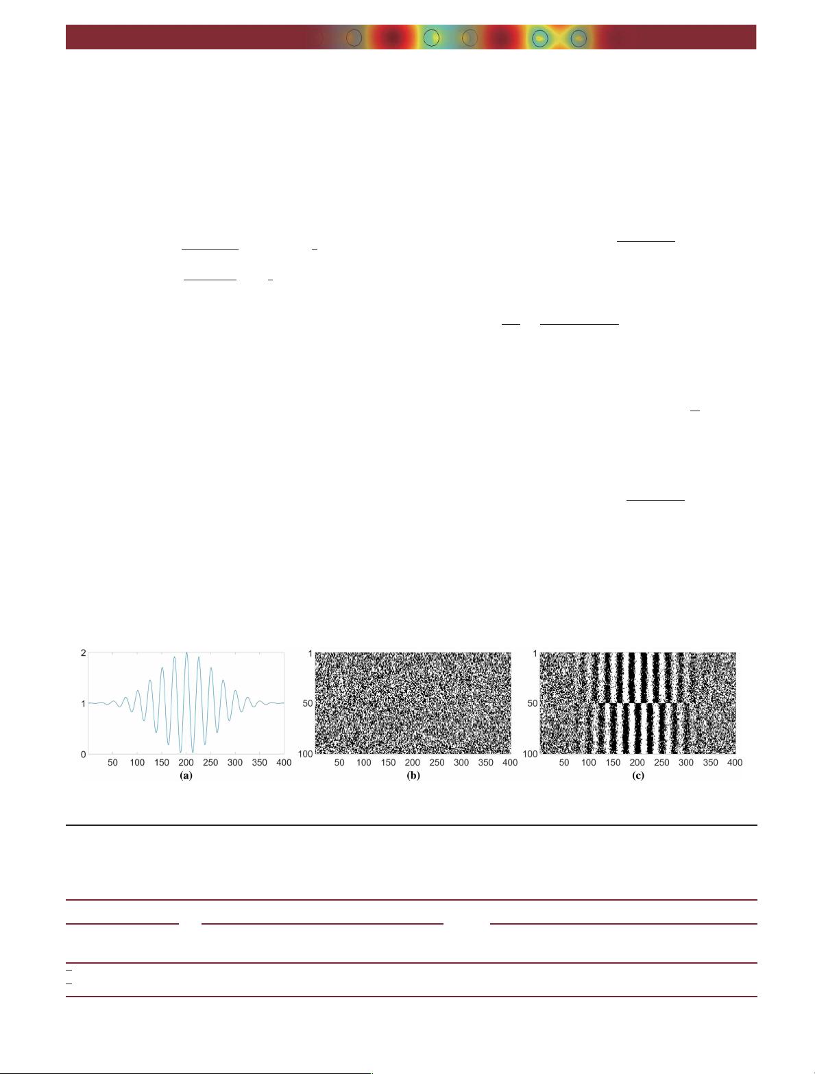
Figure 2 provides an intuitive illustration of different projection
matrices (N 401, L 100) for the one-dimensional signal
in Fig. 2(a). Figure 2(b) shows the conventional random pro-
jection matrix with Bernoulli sampling. Figure 2(c) illustrates
the TACS projection matrix. In Figs. 2(b) and 2(c), the white
and black pixels have the values of 1 and 0, respectively. Note
that the TACS projection matrix extracts some structural char-
acteristics of the original signal in Fig. 2(a), while the random
projection matrix does not. In particular, the TACS projection
matrix includes two sub-matrices. The top-half and bottom-
half sub-matrices respectively capture the structural character-
istics of the signal components beyond and below the threshold
values. Thus, the overall compressive measurements capture the
features of the entire signal.
Next, we use the design rule described in Subsection 2.A to
assess the merit of the TACS projection matrix. Note that the
voxels in hyperspectral images represent light intensities and
thus they are always non-negative. This property will be used
in the proof. In Appendix A, the proposed TACS projection
matrix is proved to make the mean values of μ
ϒ
and μ
¯
ϒ
satisfy
the following properties:
¯μ
ϒ
Δ
max
~
ψ
j
∈ϒ
Efjh
~
ϕ
i
,
~
ψ
j
ij
2
g >
k
~
X k
2
2
2NK
2
θ
2
max
,
¯μ
¯
ϒ
Δ
max
~
ψ
j
∈
¯
ϒ
Efjh
~
ϕ
i
,
~
ψ
j
ij
2
g
≈
1
4N
ffiffiffi
2
p
μ
X
ffiffiffiffiffiffiffiffiffiffiffiffiffiffiffiffiffiffiffiffiffiffiffi
πσ
2
Λ
σ
2
X
p
1
X
N
m1
ˆ
~
ψ
m
2
, (5)
where Ef·g represents the mathematical expectation; θ
max
rep-
resents the maximum element in the coefficient vector
~
Θ; and
μ
X
, σ
2
X
correspond to the mean value and variance of
~
X , respec-
tively.
ˆ
~
ψ
m
is the mth element in the vector
ˆ
~
ψ ∈ ϒ that max-
imizes the mathematical expectation. In Appendix B ,we
further prove that if Ψ is chosen as the 2D-inverse DCT
(IDCT) basis, then Eq. (5) becomes
¯μ
ϒ
max
~
ψ
j
∈ϒ
Efjh
~
ϕ
i
,
~
ψ
j
ij
2
g >
k
~
X k
2
2
2NK
2
θ
2
max
,
¯μ
¯
ϒ
max
~
ψ
j
∈
¯
ϒ
Efjh
~
ϕ
i
,
~
ψ
j
ij
2
g ≈ 0 : (6)
Equation (6) indicates that the proposed TACS projection ma-
trix can separate μ
ϒ
and μ
¯
ϒ
in the statistical sense, thus making
it satisfy the design rule.
Fig. 2. Examples of different projection matrices (N 401, L 100) for the original signal shown in (a): (b) the random projection matrix and
(c) the TACS projection matrix.
Table 1. Comparison of Mean Values of
μ
ϒ
and
μ
¯
ϒ
Obtained by Random Projection Matrices and TACS Projection
Matrices
Signal Signal 1 with Dimension 400 × 1 Signal 2 with Dimension 2500 × 1
Projection matrix
Random
(N 400, L 50)
TACS
(N 400, L 50)
Random
(N 2500, L 120)
TACS
(N 2500, L 120)
μ
ϒ
0.30927 0.32018 0.27633 0.30408
μ
¯
ϒ
0.00405 0.00285 0.00080 0.00057
398 Vol. 8, No. 3 / March 2020 / Photonics Research
Research Article


