ax88179a原理图

AX88179A是一款高速USB 3.0以太网控制器芯片，可以支持最高5Gbps的数据传输速度。该芯片的原理图包含了多个模块，其中最重要的包括PHY模块、MAC模块、USB模块、EEPROM模块和GPIO模块等。

PHY模块主要负责处理传输介质和电气信号，实现物理层数据传输。MAC模块则用于处理上层协议的数据，包括以太网层和IP层等，实现数据帧的处理和转发。USB模块主要负责USB接口数据传输和控制，包括数据收发和USB协议处理等。EEPROM模块则可以存储和读取芯片的配置信息和数据。GPIO模块则用于控制芯片的各种输入和输出信号。

在AX88179A的原理图中，各个模块之间通过统一的内部总线来进行数据和控制信号传输。总线控制器可以进行复杂的控制和处理，实现各个模块之间的数据交互和通信。

总之，AX88179A的原理图是一个复杂的系统，由多个模块协作完成数据传输和处理任务，为用户提供高速稳定的网络连接。

相关问题

skimage图像降噪原理和代码

skimage（scikit-image）是一个基于Python的开源图像处理库，其中包含了许多常见的图像处理算法和函数。skimage中提供了几种图像降噪的方法，下面详细介绍其中的一种方法：基于总变差（Total Variation）的降噪方法。

总变差降噪法是一种常用的图像降噪方法，其原理是通过对图像像素值的差异进行约束，使图像的像素值变化越小越好。具体而言，该方法使用了L2范数和L1范数之间的平衡，其中L2范数用于平滑化图像，L1范数用于保留图像边缘信息。

下面是使用skimage中的total_variation_denoising函数进行图像降噪的示例代码：

import matplotlib.pyplot as plt
from skimage import data, img_as_float
from skimage.filters import total_variation_denoising

# 加载示例图像
image = img_as_float(data.camera())

# 添加高斯噪声
from skimage.util import random_noise
image = random_noise(image, mode='gaussian', var=0.01)

# 进行降噪处理
denoised = total_variation_denoising(image, weight=0.1, max_iter=100)

# 显示结果
fig, axes = plt.subplots(nrows=1, ncols=3, figsize=(8, 5))
ax = axes.ravel()
ax[0].imshow(image, cmap=plt.cm.gray)
ax[0].set_title('Original')
ax[1].imshow(denoised, cmap=plt.cm.gray)
ax[1].set_title('Total Variation Denoising')
ax[2].imshow(image - denoised, cmap=plt.cm.gray)
ax[2].set_title('Difference')
for a in ax:
    a.axis('off')
plt.tight_layout()
plt.show()

该示例代码中，首先使用img_as_float函数将示例图像转换为浮点数格式，然后添加高斯噪声。接着，使用total_variation_denoising函数进行降噪处理，其中weight参数用于调整L2范数和L1范数的平衡，max_iter参数用于控制迭代次数。最后，使用Matplotlib库将原始图像、降噪后的图像以及两者之间的差异显示出来。

需要注意的是，总变差降噪法虽然可以在一定程度上降低图像的噪声，但也会对图像的细节信息造成一定的影响，因此需要根据实际情况进行调整。

如何利用代码画一个深度学习的工作原理图

要画深度学习的工作原理图，可以使用各种绘图工具，如Microsoft Visio、Lucidchart、Draw.io等等。以下是一些步骤和代码示例来绘制一个简单的神经网络的工作原理图。

步骤1：定义节点和连接线
首先，我们需要定义神经网络的节点和连接线。节点代表神经网络中的每个神经元，连接线代表每个神经元之间的连接。我们可以使用Visio、Lucidchart等工具手动绘制这些节点和连接线。但是，如果我们想自动化绘制这些节点和连接线，我们可以使用Python代码来实现。

以下是一个使用Python的Matplotlib库绘制神经网络的示例代码：

import matplotlib.pyplot as plt

def draw_neural_net(ax, left, right, bottom, top, layer_sizes):
    '''
    Draw a neural network cartoon using matplotilb.
    
    :usage:
        fig, ax = plt.subplots(figsize=(12, 12))
        draw_neural_net(ax, .1, .9, .1, .9, [4, 7, 2])
    
    :param ax: matplotlib `axes` object
        The axes object to draw the plot on, eg. to overlay multiple plots.
    
    :param left: float
        The center of the leftmost node(s) will be placed here.
    
    :param right: float
        The center of the rightmost node(s) will be placed here.
    
    :param bottom: float
        The center of the bottommost node(s) will be placed here.
    
    :param top: float
        The center of the topmost node(s) will be placed here.
    
    :param layer_sizes: list of int
        List of layer sizes, including input and output dimensionality.
    
    :return: None
    '''
    n_layers = len(layer_sizes)
    v_spacing = (top - bottom)/float(max(layer_sizes))
    h_spacing = (right - left)/float(len(layer_sizes) - 1)
    # Nodes
    for n, layer_size in enumerate(layer_sizes):
        layer_top = v_spacing*(layer_size - 1)/2. + (top + bottom)/2.
        for m in range(layer_size):
            circle = plt.Circle((n*h_spacing + left, layer_top - m*v_spacing), v_spacing/4.,
                                color='w', ec='k', zorder=4)
            ax.add_artist(circle)
    # Edges
    for n, (layer_size_a, layer_size_b) in enumerate(zip(layer_sizes[:-1], layer_sizes[1:])):
        layer_top_a = v_spacing*(layer_size_a - 1)/2. + (top + bottom)/2.
        layer_top_b = v_spacing*(layer_size_b - 1)/2. + (top + bottom)/2.
        for m in range(layer_size_a):
            for o in range(layer_size_b):
                line = plt.Line2D([n*h_spacing + left, (n + 1)*h_spacing + left],
                                  [layer_top_a - m*v_spacing, layer_top_b - o*v_spacing], c='k')
                ax.add_artist(line)

步骤2：绘制神经网络
现在我们可以使用上面的代码来绘制神经网络。以下是一个使用上面的代码绘制一个简单的神经网络的示例：

fig, ax = plt.subplots(figsize=(12, 12))

# Define the coordinates of the left, right, bottom and top of the figure
left, right, bottom, top = 0.1, 0.9, 0.1, 0.9

# Define the size of each layer in the neural network
layer_sizes = [4, 5, 3, 2]

# Draw the neural network
draw_neural_net(ax, left, right, bottom, top, layer_sizes)

# Show the plot
plt.show()

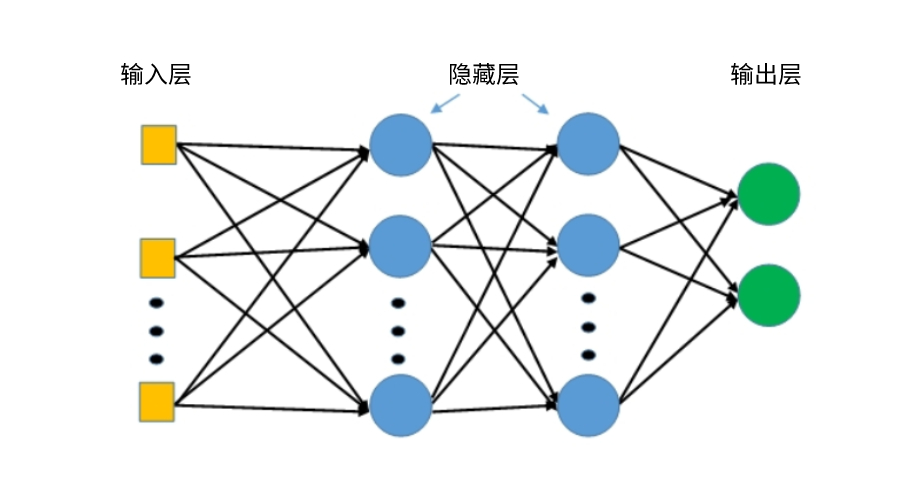
这将绘制一个包含4个输入神经元、5个隐藏神经元、3个隐藏神经元和2个输出神经元的神经网络。你可以根据你的需求更改层数和神经元数量。

你也可以使用其他库如TensorFlow、Keras等来绘制神经网络。这些库提供了专用的函数和方法来绘制神经网络。