Deep Residual Output Layers for Neural Language Generation
discussed so far, assuming a fixed |V|, d, d
h
:
C
tied
< C
bilinear
≤ C
dual
≤ C
base
, (6)
where
C
tied
,
C
base
,
C
bilinear
and
C
dual
respectively corre-
spond to the number of dedicated parameters of an output
layer with (Eq. 2) and without (Eq. 1) weight tying, using
the bilinear mapping (Eq. 3) and the dual nonlinear mapping
(Eq. 5) which are assumed to be nonzero except C
tied
.
Given this analysis, we identify and aim to address the
following limitations of the previously proposed output layer
parameterisations for language generation:
(a)
Shallow modeling of the label space. Output labels
are mapped into the joint space with a single (possibly
nonlinear) projection. Its power can only be increased
by increasing the dimensionality of the joint space.
(b)
Tendency to overfit. Increasing the dimensionality of
the joint space and thus the power of the output classi-
fier can lead to undesirable effects such as overfitting
in certain language generation tasks, which limits its
applicability to arbitrary domains.
3. Deep Residual Output Layers
To address the aforementioned limitations we propose a
deep residual output layer architecture for neural language
generation which performs deep modeling of the structure
of the output space while it preserves acquired information
and avoids overfitting. Our formulation adopts the gen-
eral form and the basic principles of previous output layer
parametrizations which aim to capture the output structure
explicitly in Section 2.3, namely (i) learning rich output
structure, (ii) controlling the output layer capacity indepen-
dently of the dimensionality of the vocabulary, the encoder
and the word embedding, and, lastly, (iii) avoiding costly
label-set-size dependent parameterisations.
3.1. Overview
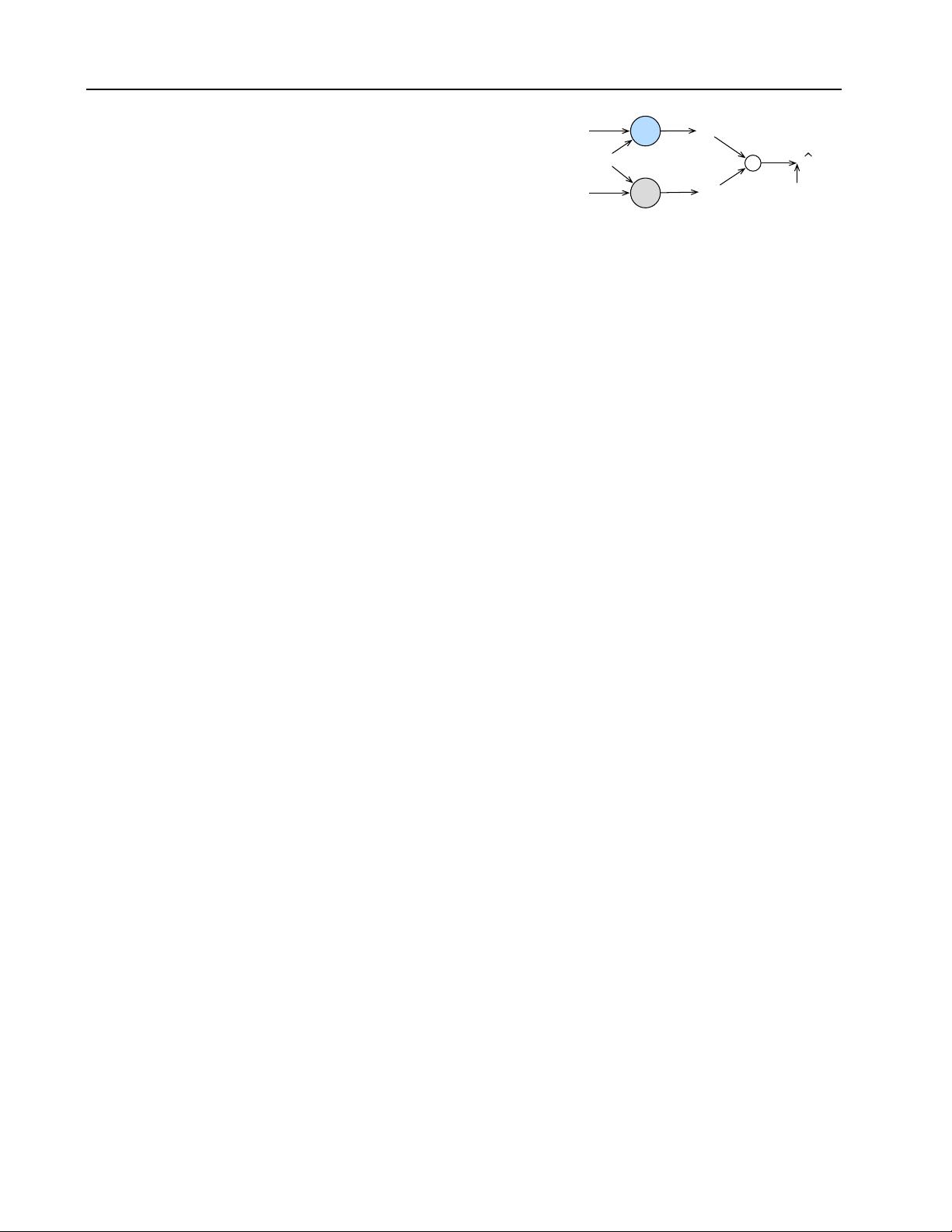
A general overview of the proposed architecture for neural
language generation is displayed in Fig. 1. We base our
output layer formulation starting on the general form of the
dual nonlinear mapping of Eq. 4:
p(y
t
|y
t−1
1
) ∝ exp
g
out
(E)g
in
(h
t
) + b
. (7)
The input network
g
in
(·)
takes as input a sequence of words
represented by their input word embeddings
E
which have
been encoded in a context representation
h
t
for the given
time step
t
. The output or label network
g
out
(·)
takes as
input the word(s) describing each possible output label and
encodes them in a label embedding
E
(k)
where
k
is the
depth of the label encoder network. Next, we define these
two proposed networks, and then we discuss how the model
is trained and how it relates to previous output layers.
g
out
E
g
in
w
1
, w
2
, …, w
T
w
1
, w
2
, …, w
|V|
E
h
t
(k)
b
y
.
Input text
Output text
Figure 1. General overview of the proposed architecture.
3.2. Label Encoder Network
For language generation tasks, the output labels are each a
word in the vocabulary
V
. We assume that these labels are
represented with their associated word embedding, which is
a row in
E
. In general, there may be additional information
about each label, such as dictionary entries, cross-lingual
resources, or contextual information, in which case we can
add an initial encoder for these descriptions which outputs
a label embedding matrix
E
0
∈ IR
|V|×d
. In this paper we
make the simplifying assumption that
E
0
= E
and leave the
investigation of additional label information to future work.
3.2.1. LEARNING OUTPUT STRUCTURE
To obtain a label representation which is able to encode rich
output space structure, we define the
g
out
(·)
function to be
a deep neural network with
k
layers which takes the label
embedding
E
as input and outputs its deep label mapping
at the last layer, g
out
(E) = E
(k)
, as follows:
E
(k)
= f
(k)
out
(E
(k−1)
), (8)
where
k
is the depth of the network and each function
f
(i)
out
(·)
at the
i
th
layer is a nonlinear projection of the following
form:
f
(i)
out
(E
(i−1)
) = σ(E
(i−1)
U
(i)
+ b
(i)
u
), (9)
where
σ(·)
is a nonlinear activation function such as
ReLU
or
Tanh
, and the matrix
U
(i)
∈ IR
d×d
j
and the bias
b
(i)
u
∈
IR
d
j
are the linear projection of the encoded outputs at the
i
th
layer. Note that when we restrict the above label network
to have one layer depth the projection is equivalent to the
label mapping from previous work in Eq. 5.
3.2.2. PRESERVING INFORMATION
The multiple layers of projections in Eq. 8 force the relation-
ship between word embeddings
E
and label embeddings
E
(k)
to be highly nonlinear. To preserve useful informa-
tion from the original word embeddings and to facilitate
the learning of the label network we add a skip connection
directly to the input embedding. Optionally, for very deep
label networks, we also add a residual connection to previ-
ous layers as in (He et al., 2016). With these additions the
projection at the k
th
layer becomes:
E
(k)
= f
(k)
out
(E
(k−1)
) + E
(k−1)
+ E (10)


