
that the most discriminative spatial patterns of aging are sparse.
Figure 2 shows the classification result using voxels selected by
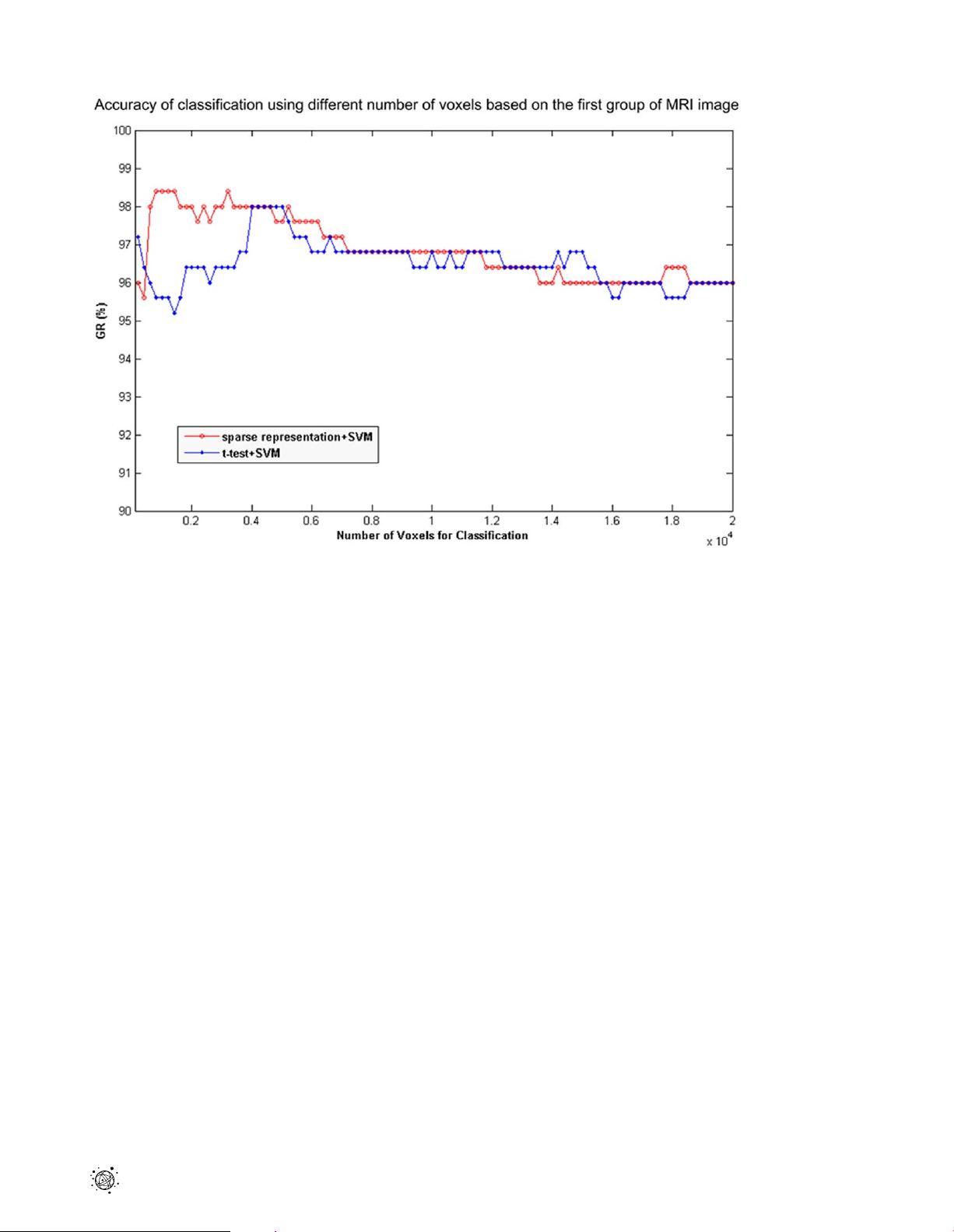
sparse representation according to the ordering of the voxels: a
decreasing arrangement by weight as determined by sparse
representation. For a better understanding of the effects of the
two steps of the proposed method, the voxels arranged according
to the score of a t-test filter in the first step were also used for
classification. The result is displayed in Figure 2. The sparse
method has two advantages over a t-test; one advantage is its high
classification rate (98.4%), and the other advantage is the ability to
achieve this accuracy using as few voxels as possible (about 1000
voxels).
Figure 2 indicates that generalization rate (GR) of the
classification reaches its peak at 98.4% using only 1000 voxels
identified by the sparse representation method, while the
classification accuracy using the structural connection is 87.46%
[38]. This is a very high rate of accuracy compared with the state-
of-art technology. However, additional voxels can degrade the
performance of the classifier. In contrast, the GR of classification
based on a t-test reaches its peak when more voxels were needed.
Because the proposed method includes a t-test filter, the chosen
voxels are included in the voxels directly selected by a t-test when
selecting for the same amount of voxels. Thus, with sufficient
confidence, the second step of proposed method predominantly
contributes to higher classification accuracy.
We aimed to providing an overview of the weightings of the
entire brain, and thus, projected the t-test values of the first 20000
voxels and weightings of the sparse method onto the human brain
map. These results are shown in Figure 3. In particular, we
focused on the weightings of the brain regions in green circles.
These regions were weighted more by the sparse method and will
be further discussed in our study.
When used as a classifier, SVM will give each subject a score
according to its distance from the separating hyperplane. The
SVM scores were closely related to chronological age. The
Pearson correlation coefficient of the SVM score and chronolog-
ical age has been studied and found to be r = 0.9339 for sparse
representation + SVM and r = 0.9279 for t-test + SVM.
The final covariance patterns constructed by the first group of
MRI data were then applied to the second group of MRI images.
These classification results are shown in Figure 4. The graph on
the left is classification results of the spatial pattern selected by the
sparse representation (GR: 96.4%, SS: 95.8%, SC: 96.8%), while
the graph on the right represents the classification results
according to a t-test (GR: 91.1%, SS: 91.7%, SC: 90.6%).
Discriminative Spatial Patterns of Aging
Figure 5 shows the final spatial patterns of aging, which were
extracted by sparse representation with the goal of facilitating
analysis. The representative regions were defined from the spatial
patterns according to the cluster size. Their anatomical labels and
Montreal Neurological Institute (MNI) coordinates obtained by
the xJview MATLAB toolbox are summarized in Table 1. For a
comparison with the final covariance patterns, Figure 6 shows the
results of the statistical t-test between GM volume of the young
and the old.
By comparing Figure 5 with Figure 6, we can distinguish
between the brain regions selected by the second step of sparse
representation from those selected by a t-test filter. In addition to
the four clusters selected by a t-test, the other four clusters were
Figure 2. Classification results of the sparse representation and t-test filter (group 1). The voxels were ordered according to weight given
by sparse representation and score of two-sample t-test. The x-axis is the number of voxels used for the classification, and the y-axis is the
classification accuracy (GR).
doi:10.1371/journal.pone.0036147.g002
Sparse Representation of Brain Aging
PLoS ONE | www.plosone.org 3 May 2012 | Volume 7 | Issue 5 | e36147
剩余12页未读,继续阅读

weixin_38665668
- 粉丝: 4
- 资源: 941
 我的内容管理
展开
我的内容管理
展开


最新资源
- 十种常见电感线圈电感量计算公式详解
- 军用车辆:CAN总线的集成与优势
- CAN总线在汽车智能换档系统中的作用与实现
- CAN总线数据超载问题及解决策略
- 汽车车身系统CAN总线设计与应用
- SAP企业需求深度剖析:财务会计与供应链的关键流程与改进策略
- CAN总线在发动机电控系统中的通信设计实践
- Spring与iBATIS整合:快速开发与比较分析
- CAN总线驱动的整车管理系统硬件设计详解
- CAN总线通讯智能节点设计与实现
- DSP实现电动汽车CAN总线通讯技术
- CAN协议网关设计:自动位速率检测与互连
- Xcode免证书调试iPad程序开发指南
- 分布式数据库查询优化算法探讨
- Win7安装VC++6.0完全指南:解决兼容性与Office冲突
- MFC实现学生信息管理系统:登录与数据库操作
资源上传下载、课程学习等过程中有任何疑问或建议,欢迎提出宝贵意见哦~我们会及时处理!
点击此处反馈


