
4
Downstream
task
Encoder
Fine-tune
Label
Prediction
head
Encoder
Pre-train
SSL task
Parameter
Downstream
task
Representation
Encoder
Prediction
head
Unsupervised pre-training
Unsupervised representation learning
Auxiliary learning
Encoder SSL task
Auxiliary
SSL task
Main task
Label
( )
Label
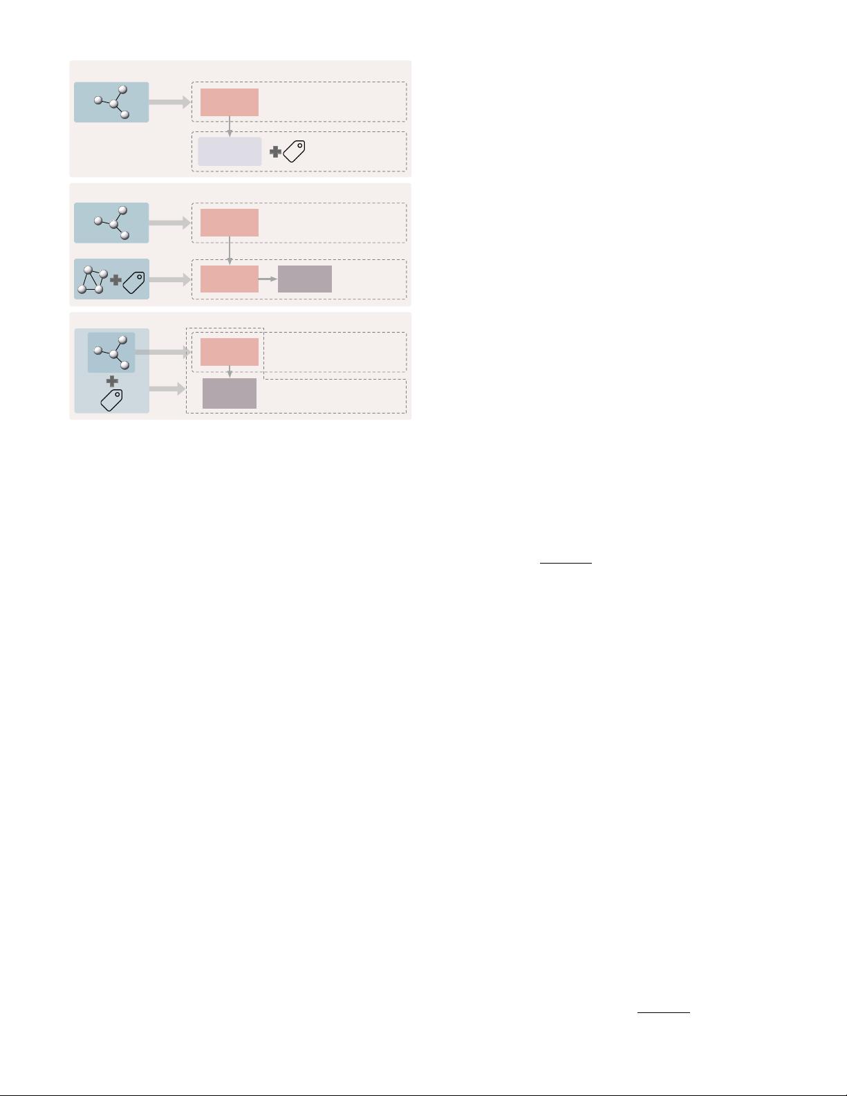
Fig. 3. Paradigms for self-supervised learning. Top:in unsupervised rep-
resentation learning, graphs only are used to train the encoder through
the self-supervised task. The learned representations are fixed and
used in downstream tasks such as linear classification and clustering.
Middle: unsupervised pre-training trains the encoder with unlabeled
graphs by the self-supervised task. The pre-trained encoder’s parame-
ters are then used as the initialization of the encoder used in supervised
fine-tuning for downstream tasks. Bottom: in auxiliary learning, an aux-
iliary task with self-supervision is included to help learn the supervised
main task. The encoder is trained through both the main task and the
auxiliary task simultaneously.
training graphs, contrastive learning aims to learn one or
more encoders such that representations of similar graph
instances agree with each other, and that representations
of dissimilar graph instances disagree with each other. We
unify existing approaches to constructing contrastive learn-
ing tasks into a general framework that learns to discrimi-
nate jointly sampled view pairs (e.g. two views belonging to
the same instance) from independently sampled view pairs
(e.g. views belonging to different instances). In particular,
we obtain multiple views from each graph in the training
dataset by applying different transformations. Two views
generated from the same instance are usually considered
as a positive pair and two views generated from different
instances are considered as a negative pair. The agreement
is usually measured by metrics related to the mutual infor-
mation between two representations.
One major difference among graph contrastive learning
methods lies in (a) the objective for discrimination task
given view representations. In addition, due to the unique
data structure of graphs, graph contrastive learning meth-
ods also differ in (b) approaches that views are obtained,
and (c) graph encoders that compute the representations of
views. A graph contrastive learning method can be deter-
mined by specifying its components (a)–(c). In this section,
we summarize graph contrastive learning methods in a
unified framework and then introduce (a)–(c) individually
used in existing studies.
3.1 Overview of Contrastive Learning Framework
In general, key components that specify a contrastive learn-
ing framework include transformations that compute mul-
tiple views from each given graph, encoders that compute
the representation for each view, and the learning objective
to optimize parameters in encoders. An overview of the
framework is shown in Figure 4. Concretely, given a graph
(A, X) as a random variable distributed from P, multiple
transformations T
1
, · · · , T
k
are applied to obtain different
views w
1
, · · · , w
k
of the graph. Then, a set of encoding net-
works f
1
, · · · , f
k
take corresponding views as their inputs
and output the representations h
1
, · · · , h
k
of the graph from
each views. Formally, we have
w
i
= T
i
(A, X), (6)
h
i
= f
i
(w
i
), i = 1, · · · , k. (7)
We assume w
i
= (
ˆ
A
i
,
ˆ
X
i
) = T
i
(A, X) in this survey since
existing contrastive methods consider their views as graphs.
However, note that not all views w
i
are necessarily graphs or
sub-graphs in a general sense. In addition, certain encoders
can be identical to each other or share their weights.
During training, the contrastive objective aims to train
encoders to maximize the agreement between view rep-
resentations computed from the same graph instance. The
agreement is usually measured by the mutual information
I(h
i
, h
j
) between a pair of representations h
i
and h
j
. We
formalize the contrastive objective as
max
{f
i
}
k
i=1
1
P
i6=j
σ
ij
X
i6=j
σ
ij
I(h
i
, h
j
)
, (8)
where σ
ij
∈ {0, 1}, and σ
ij
= 1 if the mutual information
is computed between h
i
and h
j
, and σ
ij
= 0 otherwise,
and h
i
and h
j
are considered as two random variables
belonging to either a joint distribution or the product of two
marginals. To enable efficient computation of the mutual
information, certain estimators
b
I of the the mutual informa-
tion are usually used instead as the learning objective. Note
that some contrastive methods apply projection heads [9, 42]
to the representations. For the sake of uniformity, we con-
sider such projection heads as parts of the computation in
the mutual information estimation.
During inference, one can either use a single trained
encoder to compute the representation or a combination of
multiple view representations such as the linear combina-
tion or the concatenation as the final representation of a
given graph. Three examples of using encoders in different
ways during inference are illustrated in Figure 5.
3.2 Contrastive Objectives
3.2.1 Mutual Information Estimation
Given a pair of random variables (x, y), the mutual infor-
mation I(x, y) measures the information that x and y share,
given by
I(x, y) = D
KL
(p(x, y)||p(x)p(y)) (9)
= E
p(x,y)
log
p(x, y)
p(x)p(y)
, (10)
剩余16页未读,继续阅读

syp_net
- 粉丝: 158
- 资源: 1187
 我的内容管理
展开
我的内容管理
展开


最新资源
- 多模态联合稀疏表示在视频目标跟踪中的应用
- Kubernetes资源管控与Gardener开源软件实践解析
- MPI集群监控与负载平衡策略
- 自动化PHP安全漏洞检测:静态代码分析与数据流方法
- 青苔数据CEO程永:技术生态与阿里云开放创新
- 制造业转型: HyperX引领企业上云策略
- 赵维五分享:航空工业电子采购上云实战与运维策略
- 单片机控制的LED点阵显示屏设计及其实现
- 驻云科技李俊涛:AI驱动的云上服务新趋势与挑战
- 6LoWPAN物联网边界路由器:设计与实现
- 猩便利工程师仲小玉:Terraform云资源管理最佳实践与团队协作
- 类差分度改进的互信息特征选择提升文本分类性能
- VERITAS与阿里云合作的混合云转型与数据保护方案
- 云制造中的生产线仿真模型设计与虚拟化研究
- 汪洋在PostgresChina2018分享:高可用 PostgreSQL 工具与架构设计
- 2018 PostgresChina大会:阿里云时空引擎Ganos在PostgreSQL中的创新应用与多模型存储
资源上传下载、课程学习等过程中有任何疑问或建议,欢迎提出宝贵意见哦~我们会及时处理!
点击此处反馈


