没有合适的资源?快使用搜索试试~ 我知道了~
首页[斯坦福大学]隐马尔科夫模型.pdf
资源详情
资源评论
资源推荐
Speech and Language Processing. Daniel Jurafsky & James H. Martin. Copyright
c
2019. All
rights reserved. Draft of October 2, 2019.
CHAPTER
A
Hidden Markov Models
Chapter 8 introduced the Hidden Markov Model and applied it to part of speech
tagging. Part of speech tagging is a fully-supervised learning task, because we have
a corpus of words labeled with the correct part-of-speech tag. But many applications
don’t have labeled data. So in this chapter, we introduce the full set of algorithms for
HMMs, including the key unsupervised learning algorithm for HMM, the Forward-
Backward algorithm. We’ll repeat some of the text from Chapter 8 for readers who
want the whole story laid out in a single chapter.
A.1 Markov Chains
The HMM is based on augmenting the Markov chain. A Markov chain is a model
Markov chain
that tells us something about the probabilities of sequences of random variables,
states, each of which can take on values from some set. These sets can be words, or
tags, or symbols representing anything, like the weather. A Markov chain makes a
very strong assumption that if we want to predict the future in the sequence, all that
matters is the current state. The states before the current state have no impact on the
future except via the current state. It’s as if to predict tomorrow’s weather you could
examine today’s weather but you weren’t allowed to look at yesterday’s weather.
WARM
3
HOT
1
COLD
2
.8
.6
.1
.1
.3
.6
.1
.1
.3
charming
uniformly
are
.1
.4
.5
.5
.5
.2
.6
.2
(a) (b)
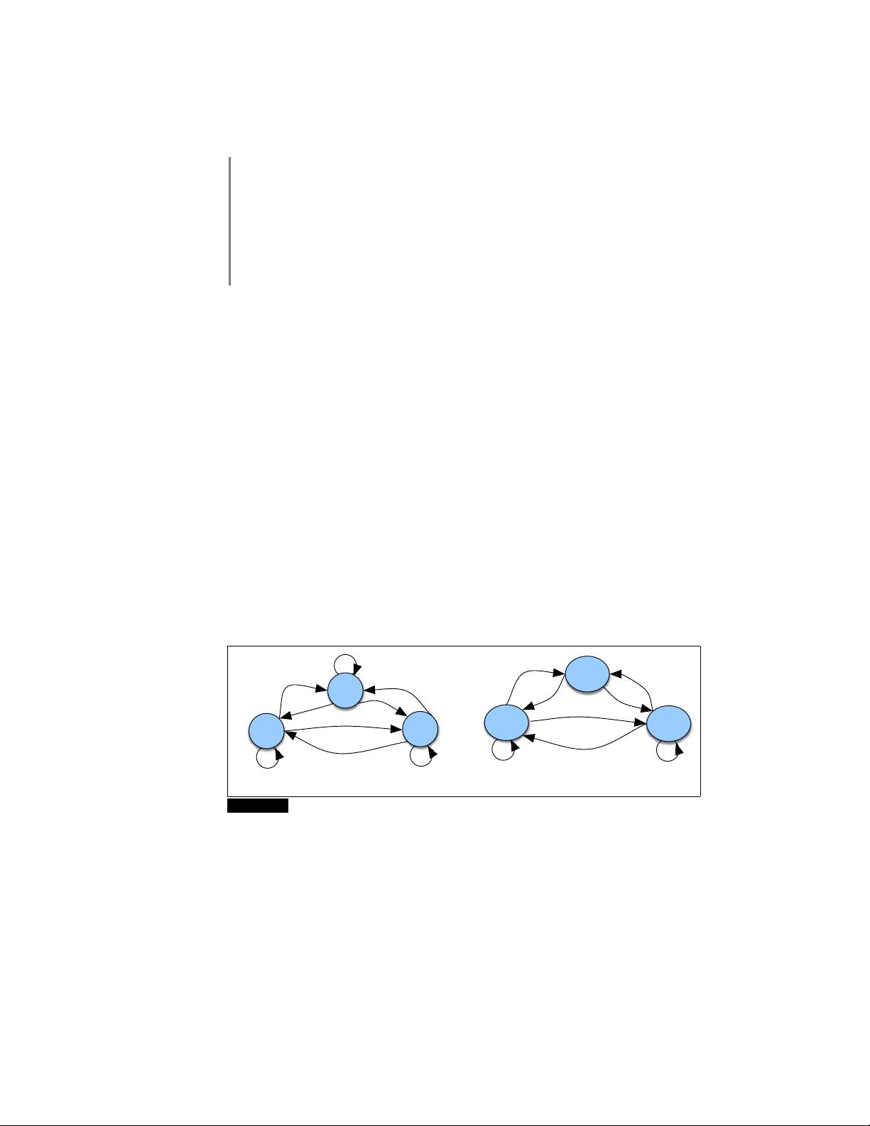
Figure A.1 A Markov chain for weather (a) and one for words (b), showing states and
transitions. A start distribution π is required; setting π = [0.1, 0.7, 0.2] for (a) would mean a
probability 0.7 of starting in state 2 (cold), probability 0.1 of starting in state 1 (hot), etc.
More formally, consider a sequence of state variables q
1
,q
2
,...,q
i
. A Markov
model embodies the Markov assumption on the probabilities of this sequence: that
Markov
assumption
when predicting the future, the past doesn’t matter, only the present.
Markov Assumption: P(q
i
= a|q
1
...q
i−1
) = P(q
i
= a|q
i−1
) (A.1)
Figure A.1a shows a Markov chain for assigning a probability to a sequence of
weather events, for which the vocabulary consists of HOT, COLD, and WARM. The
states are represented as nodes in the graph, and the transitions, with their probabil-
ities, as edges. The transitions are probabilities: the values of arcs leaving a given
2 APPENDIX A • HIDDEN MARKOV MODELS
state must sum to 1. Figure A.1b shows a Markov chain for assigning a probabil-
ity to a sequence of words w
1
...w
n
. This Markov chain should be familiar; in fact,
it represents a bigram language model, with each edge expressing the probability
p(w
i
|w
j
)! Given the two models in Fig. A.1, we can assign a probability to any
sequence from our vocabulary.
Formally, a Markov chain is specified by the following components:
Q = q
1
q
2
...q
N
a set of N states
A = a
11
a
12
...a
n1
...a
nn
a transition probability matrix A, each a
i j
represent-
ing the probability of moving from state i to state j, s.t.
P
n
j=1
a
i j
= 1 ∀i
π = π
1
,π
2
,...,π
N
an initial probability distribution over states. π
i
is the
probability that the Markov chain will start in state i.
Some states j may have π
j
= 0, meaning that they cannot
be initial states. Also,
P
n
i=1
π
i
= 1
Before you go on, use the sample probabilities in Fig. A.1a (with π = [.1,.7.,2])
to compute the probability of each of the following sequences:
(A.2) hot hot hot hot
(A.3) cold hot cold hot
What does the difference in these probabilities tell you about a real-world weather
fact encoded in Fig. A.1a?
A.2 The Hidden Markov Model
A Markov chain is useful when we need to compute a probability for a sequence
of observable events. In many cases, however, the events we are interested in are
hidden: we don’t observe them directly. For example we don’t normally observe
hidden
part-of-speech tags in a text. Rather, we see words, and must infer the tags from the
word sequence. We call the tags hidden because they are not observed.
A hidden Markov model (HMM) allows us to talk about both observed events
Hidden
Markov model
(like words that we see in the input) and hidden events (like part-of-speech tags) that
we think of as causal factors in our probabilistic model. An HMM is specified by
the following components:
Q = q
1
q
2
...q
N
a set of N states
A = a
11
...a
i j
...a
NN
a transition probability matrix A, each a
i j
representing the probability
of moving from state i to state j , s.t.
P
N
j=1
a
i j
= 1 ∀i
O = o
1
o
2
...o
T
a sequence of T observations, each one drawn from a vocabulary V =
v
1
,v
2
,...,v
V
B = b
i
(o
t
) a sequence of observation likelihoods, also called emission probabili-
ties, each expressing the probability of an observation o
t
being generated
from a state i
π = π
1
,π
2
,...,π
N
an initial probability distribution over states. π
i
is the probability that
the Markov chain will start in state i. Some states j may have π
j
= 0,
meaning that they cannot be initial states. Also,
P
n
i=1
π
i
= 1
A.2 • THE HIDDEN MARKOV MODEL 3
A first-order hidden Markov model instantiates two simplifying assumptions.
First, as with a first-order Markov chain, the probability of a particular state depends
only on the previous state:
Markov Assumption: P(q
i
|q
1
...q
i−1
) = P(q
i
|q
i−1
) (A.4)
Second, the probability of an output observation o
i
depends only on the state that
produced the observation q
i
and not on any other states or any other observations:
Output Independence: P(o
i
|q
1
...q
i
,...,q
T
,o
1
,...,o
i
,...,o
T
) = P(o
i
|q
i
) (A.5)
To exemplify these models, we’ll use a task invented by Jason Eisner (2002).
Imagine that you are a climatologist in the year 2799 studying the history of global
warming. You cannot find any records of the weather in Baltimore, Maryland, for
the summer of 2020, but you do find Jason Eisner’s diary, which lists how many ice
creams Jason ate every day that summer. Our goal is to use these observations to
estimate the temperature every day. We’ll simplify this weather task by assuming
there are only two kinds of days: cold (C) and hot (H). So the Eisner task is as
follows:
Given a sequence of observations O (each an integer representing the
number of ice creams eaten on a given day) find the ‘hidden’ sequence
Q of weather states (H or C) which caused Jason to eat the ice cream.
Figure A.2 shows a sample HMM for the ice cream task. The two hidden states
(H and C) correspond to hot and cold weather, and the observations (drawn from the
alphabet O = {1,2,3}) correspond to the number of ice creams eaten by Jason on a
given day.
π = [.8,.2]
COLD
2
HOT
1
B
2
P(1 | COLD) .5
P(2 | COLD) = .4
P(3 | COLD) .1
.5
.6
.5
.4
P(1 | HOT) .2
P(2 | HOT) = .4
P(3 | HOT) .4
B
1
Figure A.2 A hidden Markov model for relating numbers of ice creams eaten by Jason (the
observations) to the weather (H or C, the hidden variables).
An influential tutorial by Rabiner (1989), based on tutorials by Jack Ferguson in
the 1960s, introduced the idea that hidden Markov models should be characterized
by three fundamental problems:
Problem 1 (Likelihood): Given an HMM λ = (A, B) and an observation se-
quence O, determine the likelihood P(O|λ).
Problem 2 (Decoding): Given an observation sequence O and an HMM λ =
(A,B), discover the best hidden state sequence Q.
Problem 3 (Learning): Given an observation sequence O and the set of states
in the HMM, learn the HMM parameters A and B.
We already saw an example of Problem 2 in Chapter 8. In the next two sections
we introduce the Forward and Forward-Backward algorithms to solve Problems 1
and 3 and give more information on Problem 2
4 APPENDIX A • HIDDEN MARKOV MODELS
A.3 Likelihood Computation: The Forward Algorithm
Our first problem is to compute the likelihood of a particular observation sequence.
For example, given the ice-cream eating HMM in Fig. A.2, what is the probability
of the sequence 3 1 3? More formally:
Computing Likelihood: Given an HMM λ = (A,B) and an observa-
tion sequence O, determine the likelihood P(O|λ).
For a Markov chain, where the surface observations are the same as the hidden
events, we could compute the probability of 3 1 3 just by following the states labeled
3 1 3 and multiplying the probabilities along the arcs. For a hidden Markov model,
things are not so simple. We want to determine the probability of an ice-cream
observation sequence like 3 1 3, but we don’t know what the hidden state sequence
is!
Let’s start with a slightly simpler situation. Suppose we already knew the weather
and wanted to predict how much ice cream Jason would eat. This is a useful part
of many HMM tasks. For a given hidden state sequence (e.g., hot hot cold), we can
easily compute the output likelihood of 3 1 3.
Let’s see how. First, recall that for hidden Markov models, each hidden state
produces only a single observation. Thus, the sequence of hidden states and the
sequence of observations have the same length.
1
Given this one-to-one mapping and the Markov assumptions expressed in Eq. A.4,
for a particular hidden state sequence Q = q
0
,q
1
,q
2
,...,q
T
and an observation se-
quence O = o
1
,o
2
,...,o
T
, the likelihood of the observation sequence is
P(O|Q) =
T
Y
i=1
P(o
i
|q
i
) (A.6)
The computation of the forward probability for our ice-cream observation 3 1 3 from
one possible hidden state sequence hot hot cold is shown in Eq. A.7. Figure A.3
shows a graphic representation of this computation.
P(3 1 3|hot hot cold) = P(3|hot)× P(1|hot) × P(3|cold) (A.7)
coldhot
3
.4
hot
1 3
.2 .1
Figure A.3 The computation of the observation likelihood for the ice-cream events 3 1 3
given the hidden state sequence hot hot cold.
But of course, we don’t actually know what the hidden state (weather) sequence
was. We’ll need to compute the probability of ice-cream events 3 1 3 instead by
1
In a variant of HMMs called segmental HMMs (in speech recognition) or semi-HMMs (in text pro-
cessing) this one-to-one mapping between the length of the hidden state sequence and the length of the
observation sequence does not hold.
剩余16页未读,继续阅读
小孩咋啦
- 粉丝: 0
- 资源: 1
上传资源 快速赚钱
- 我的内容管理 收起
- 我的资源 快来上传第一个资源
- 我的收益 登录查看自己的收益
- 我的积分 登录查看自己的积分
- 我的C币 登录后查看C币余额
- 我的收藏
- 我的下载
- 下载帮助
会员权益专享
最新资源
- RTL8188FU-Linux-v5.7.4.2-36687.20200602.tar(20765).gz
- c++校园超市商品信息管理系统课程设计说明书(含源代码) (2).pdf
- 建筑供配电系统相关课件.pptx
- 企业管理规章制度及管理模式.doc
- vb打开摄像头.doc
- 云计算-可信计算中认证协议改进方案.pdf
- [详细完整版]单片机编程4.ppt
- c语言常用算法.pdf
- c++经典程序代码大全.pdf
- 单片机数字时钟资料.doc
- 11项目管理前沿1.0.pptx
- 基于ssm的“魅力”繁峙宣传网站的设计与实现论文.doc
- 智慧交通综合解决方案.pptx
- 建筑防潮设计-PowerPointPresentati.pptx
- SPC统计过程控制程序.pptx
- SPC统计方法基础知识.pptx
资源上传下载、课程学习等过程中有任何疑问或建议,欢迎提出宝贵意见哦~我们会及时处理!
点击此处反馈
安全验证
文档复制为VIP权益,开通VIP直接复制
信息提交成功
评论0