Matlab偏微分方程求解方法

Matlab 偏微分方程求解方法

目录：

§1 Function Summary on page 10-87

§2 Initial Value Problems on page 10-88

§3 PDE Solver on page 10-89

§4 Integrator Options on page 10-92

§5 Examples” on page 10-93

§1 Function Summary

pdepe Solve initial-boundary value problems for systems of

parabolic and elliptic PDEs in one space variable and

time.

PDE Helper Function

PDE Helper Function Description

pdeval Evaluate the numerical solution of a PDE using the

output of pdepe

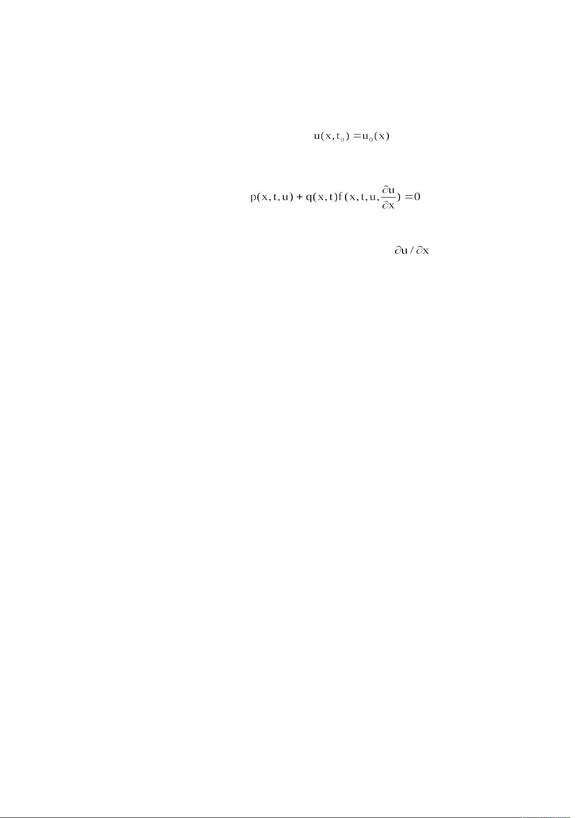
§2 Initial Value Problems

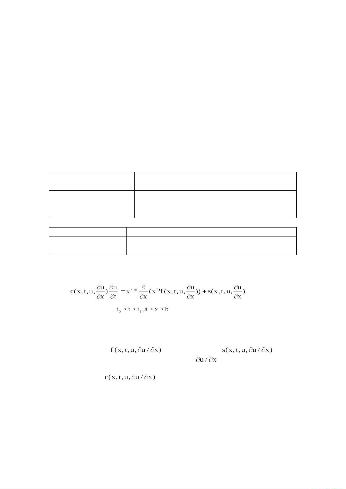
pdepe solves systems of parabolic and elliptic PDEs in one spatial

variable x and time t, of the form

partial derivatives with respect to time is restricted to multiplication by a

diagonal matrix . The diagonal elements of this matrix are

either identically zero or positive. An element that is identically zero

corresponds to an elliptic equation and otherwise to a parabolic equation.

There must be at least one parabolic equation. An element of c that

corresponds to a parabolic equation can vanish at isolated values of x if

they are mesh points.Discontinuities in c and/or s due to material

interfaces are permitted provided that a mesh point is placed at each

interface.

At the initial time t = t0, for all x the solution components satisfy initial

At the boundary x = a or x = b, for all t the solution components satisfy a

boundary condition of the form

q(x, t) is a diagonal matrix with elements that are either identically zero

problems for systems of parabolic and elliptic PDEs in the one space

variable x and time t.There must be at least one parabolic equation in the

system.

The pdepe solver converts the PDEs to ODEs using a second-order

accurate spatial discretization based on a fixed set of user-specified

nodes. The discretization method is described in [9]. The time integration

is done with ode15s. The pdepe solver exploits the capabilities of ode15s

for solving the differential-algebraic equations that arise when Equation

10-2 contains elliptic equations, and for handling Jacobians with a

specified sparsity pattern. ode15s changes both the time step and the

that at any other time. If the mesh is sufficiently fine, pdepe can find

consistent initial conditions close to the given ones. If pdepe displays a

message that it has difficulty finding consistent initial conditions, try

refining the mesh. No adjustment is necessary for elements of the initial

conditions vector that correspond to parabolic equations.

PDE Solver Syntax

The basic syntax of the solver is:

sol = pdepe(m,pdefun,icfun,bcfun,xmesh,tspan)

Note Correspondences given are to terms used in “Initial Value

Problems” on page 10-88.

cylindrical, or 2 = spherical. It corresponds to m in Equation 10-2.

pdefun: Function that defines the components of the PDE. It

where x and t are scalars, and u and dudx are vectors that approximate the

solution and its partial derivative with respect to . c, f, and s are column

vectors. c stores the diagonal elements of the matrix .

icfun: Function that evaluates the initial conditions. It has the form

u = icfun(x)

When called with an argument x, icfun evaluates and returns the initial

column vectors corresponding to p and the diagonal of q evaluated at

xl. Similarly, pr and qr correspond to xr. When m>0 and a = 0,

boundedness of the solution near x = 0 requires that the f vanish at a = 0.

pdepe imposes this boundary condition automatically and it ignores

values returned in pl and ql.

xmesh:Vector [x0, x1, ..., xn] specifying the points at which a numerical

solution is requested for every value in tspan. x0 and xn correspond to a

and b , respectively. Second-order approximation to the solution is made

on the mesh specified in xmesh. Generally, it is best to use closely spaced

mesh points where the solution changes rapidly. pdepe does not select the

tspan:Vector [t0, t1, ..., tf] specifying the points at which a solution is

respectively.

pdepe performs the time integration with an ODE solver that selects both

the time step and formula dynamically. The solutions at the points

specified in tspan are obtained using the natural continuous extension of

the integration formulas. The elements of tspan merely specify where you

want answers and the cost depends weakly on the length of tspan.