没有合适的资源?快使用搜索试试~ 我知道了~
首页曼诺拉基斯《统计与自适应信号处理》习题详解
《统计与自适应信号处理》是一本由美国作者Dimitris G. Manolakis、Vinay K. Ingle和Stephen M. Kogon合著的高级信号处理教材。本书着重于统计信号处理和随机过程理论,深入探讨了滤波器设计与应用中的自适应方法。该教材配套的课后习题答案手册由David Marden和作者团队共同编撰,旨在提供详尽的解题指导,确保读者能够理解和掌握书中的概念。 该习题答案共467页,涵盖了全书各章节的内容,解答部分采用了与书中一致的符号表示,有助于学生在学习过程中对照练习。对于那些需要用到Matlab编程的问题,手册提供了代码示例和相关图形,帮助读者实践所学的理论知识。然而,由于编写者不可能面面俱到,某些解决方案可能并不如其他问题那样详尽清晰,可能存在疏漏或错误。 为了不断改进这个答案手册,作者鼓励读者反馈,包括提供更详细的解题思路、提出新的问题建议以及对现有答案的修正。读者可以通过电子邮件联系Vinay K. Ingle教授,地址为vingle@ece.neu.edu或者直接联系他在东北大学电子工程系的办公室。定期,作者团队会根据读者的反馈更新答案,添加新问题,以满足教学需求和提升学习体验。 《统计与自适应信号处理课后习题答案》是一份实用的学习资源,不仅提供了深入的理论解析,还通过实际问题的解答,强化了学生对统计信号处理技术的理解和应用能力。对于希望深入研究该领域的学生和教师来说,这本习题答案是不可或缺的参考资料。
资源详情
资源推荐
![](https://csdnimg.cn/release/download_crawler_static/11178448/bg10.jpg)
Chapter 3
Random Variables, Random Vectors, & Stochastic Processes
3.1 Exponential Density: f
x
(x) =
1
a
e
−x/a
u(x)
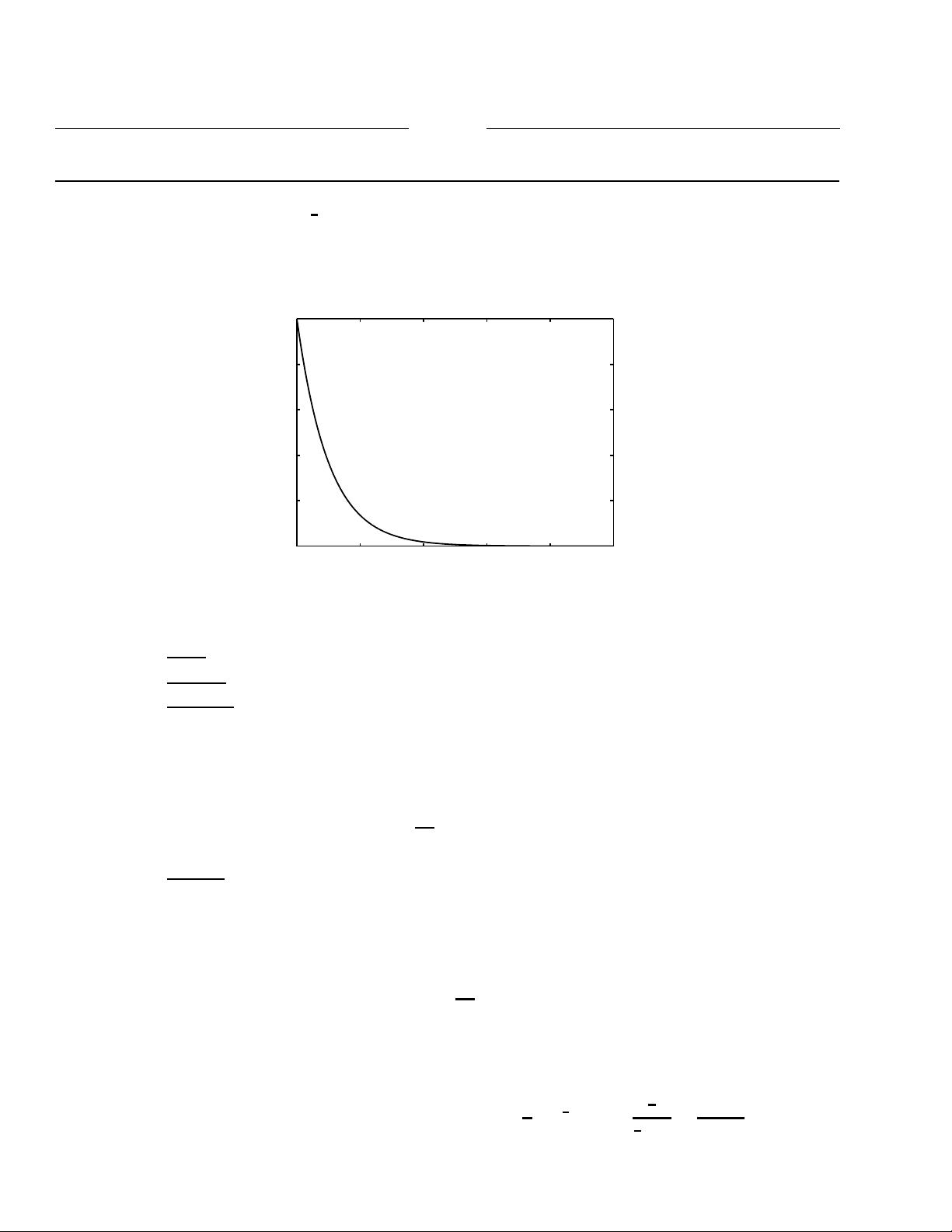
(a) Density plot for a = 1: f
x
(x) = e
−x
u(x) is shown in Figure 3.1
0 2 4 6 8 10
0
0.2
0.4
0.6
0.8
1
f
x
(x)=e
−x
u(x)
Figure 3.1: Exponential density function
(b) Moments:
i. Mean
: µ
x
=
∞
−∞
xf
x
(x)dx = 1/a = 1
ii. Variance
: σ
2
x
=
∞
−∞
(x − µ
x
)
2
f
x
(x)dx = (1/a)
2
= 1
iii. Skewness
: The third central moment is given by
γ
(3)
x
=
∞
−∞
x − µ
x
3
f
x
(
x
)
dx =
∞
0
(
x − 1
)
3
(e
−x
)dx = 2
Hence
skewness =
1
σ
3
x
γ
(3)
x
= 2 (⇒ leaning towards right)
iv. Kurtosis
: The fourth central moment is given by
γ
(4)
x
=
∞
−∞
x − µ
x
4
f
x
(
x
)
dx =
∞
0
(
x − 1
)
4
(e
−x
)dx = 9
Hence
kurtosis =
1
σ
4
x
γ
(4)
x
− 3 = 9 − 3 = 4
which means a much flatter shape compared to the Gaussian shape.
(c) Characteristic function:
x
=
E
{e
sx(ξ)
}=
∞
−∞
f
x
(x)e
sx
dx =
∞
0
1
a
e
−x(
1
a
−s)
dx =
1
a
1
a
− s
=
1
1 − as
12
![](https://csdnimg.cn/release/download_crawler_static/11178448/bg11.jpg)
Statistical and Adaptive Signal Processing - Solution Manual 13
0 2 4 6 8 10
0
0.1
0.2
0.3
0.4
0.5
f
x
(x)=xe
−x
2
u(x)
Figure 3.2: Rayleigh density function
3.2 Rayleigh density : f
x
(x) =
x
σ
2
e
−x
2
/(2σ
2
)
u(x)
(a) Density function for σ = 1: f
x
(x) = xe
−x
2
/2
u(x) is shown in Figure 3.2.
(b) Moments:
i. Mean
: µ
x
=
∞
−∞
xf
x
(x)dx =
∞
0
x
2
e
−x
2
/2
dx =
√
π/2
ii. Variance
: σ
2
x
=
∞
−∞
(x − µ
x
)
2
f
x
(x)dx =
∞
0
(x −
√
π/2)
2
xe
−x
2
/2
dx = 2 −
π
2
iii. Skewness: The third central moment is given by
γ
(3)
x
=
∞
−∞
x − µ
x
3
f
x
(
x
)
dx =
∞
0
x −
π/2
3
(xe
−x
2
/2
)dx =
1
√
2
√
π
3
−
3
√
2
√
π
Hence
skewness =
1
σ
3
x
γ
(3)
x
=
1
√
2
√
π
3
−
3
√
2
√
π
2 −
π
2
3
= . 63111 (⇒ leaning towards right)
iv. Kurtosis
: The fourth central moment is given by
γ
(4)
x
=
∞
−∞
x − µ
x
4
f
x
(
x
)
dx =
∞
0
x −
π/2
4
(xe
−x
2
/2
)dx = 8 −
3π
2
4
: Hence
kurtosis =
1
σ
4
x
γ
(4)
x
− 3 =
8 −
3π
2
4
2 −
π
2
2
− 3 = 0.2451
which means a flatter but almost a Gaussian shape.
(c) Characteristic function (σ = 1):
x
(s) =
E
{e
sx(ξ)
}=
∞
−∞
f
x
(x)e
sx
dx =
y
0
xe
−x
2
e
sx
dx
=
1
4
s
√
πe
1
4
s
2
+
1
2
+
1
4
s
√
πe
1
4
s
2
erf
1
2
s
![](https://csdnimg.cn/release/download_crawler_static/11178448/bg12.jpg)
14 Statistical and Adaptive Signal Processing - Solution Manual
3.3 Relation between r
(m)
x
and γ
(m)
x
:
γ
(m)
x
=
E
{[x(ζ ) − µ
x
]
m
}=
E
m
k=0
(−1)
k
m
k
x(ζ )
k
µ
m−k
x
=
m
k=0
(−1)
k
m
k
µ
k
x
E{x(ζ )
k
}
γ
(m)
x
=
m
k=0
(−1)
k
m
k
µ
k
x
r
(n−k)
x
Similarly
r
(m)
x
=
E
{(
x(ζ ) − µ
x
y(ζ )
+ µ
x
)
m
}=
E
m
k=0
m
k
y(ζ )
k
µ
m−k
x
=
m
k=0
m
k
µ
k
x
E
{y(ζ)
k
}
r
(m)
x
=
m
k=0
m
k
µ
k
x
γ
(n−k)
x
3.4 First four cumulants: The cumulants are given by
κ
(m)
x
,
d
m
¯
x
(
s
)
ds
m
s=0
where
¯
x
(s) = ln
¯
x
(s) = ln
E
e
sx(ζ )
= ln [
x
(s)]
and
x
(s) =
∞
m=0
s
m
m!
r
(m)
x
Thus
κ
(1)
x
=
1
x
(s)
d
x
(s)
ds
s=0
=
!
∞
m=0
s
m
m!
r
(m+1)
x
!
∞
m=0
s
m
m!
r
(m)
x
s=0
= r
(1)
x
= µ
x
= 0[
*
zero mean x(ζ )]
Similarly
κ
(2)
x
=
d
ds
!
∞
m=0
s
m
m!
r
(m+1)
x
!
∞
m=0
s
m
m!
r
(m)
x
s=0
=
!
∞
m=0
s
m
m!
r
(m+2)
x
!
∞
m=0
s
m
m!
r
(m)
x
−
!
∞
m=0
s
m
m!
r
(m+1)
x
2
!
∞
m=0
s
m
m!
r
(m)
x
2
s=0,r
(1)
x
=0
= r
(2)
x
= σ
2
x
![](https://csdnimg.cn/release/download_crawler_static/11178448/bg13.jpg)
Statistical and Adaptive Signal Processing - Solution Manual 15
κ
(3)
x
=
d
ds
!
∞
m=0
s
m
m!
r
(m+2)
x
!
∞
m=0
s
m
m!
r
(m)
x
−
!
∞
m=0
s
m
m!
r
(m+1)
x
2
!
∞
m=0
s
m
m!
r
(m)
x
2
s=0,r
(1)
x
=0
= γ
(3)
x
3.5 Random vector x(ζ ) = [x
1
(ζ ) x
2
(ζ )]
(a) Mean vector:
µ
y
= Aµ
x
=
13
−12
23
1
2
=
7
3
8
(b) Autocorrelation matrix:
y
= A
x
A
H
=
13
−12
23
40.8
0.81
1 −12
323
=
17.81.224.2
1.24.8 −1.2
24.2 −1.234.6
(c) Crosscorrelation matrix:
R
x
=
x
+ µ
x
µ
H
x
=
52.8
2.85
R
xy
= R
x
A
H
=
13.40.618.4
17.87.220.6
3.6 Let x(ζ ) be a Gaussian random vector with mean vector µ
x
and covariance matrix
x
, then the characteristic
function is
x
(
ξ
)
= exp
jξ
T
µ
x
−
1
2
ξ
T
x
ξ
Let y(ζ ) = Ax where A is a non-singular matrix. Its characteristic function is given by
y
(
ξ
)
=
E
"
e
jξ
T
y
#
=
E
"
e
jξ
T
Ax
#
=
E
"
e
j
(
A
T
ξ
)
T
x
#
= exp
$
j
A
T
ξ
T
µ
x
−
1
2
A
T
ξ
T
x
A
T
ξ
%
= exp
jξ
T
Aµ
x
−
1
2
ξ
T
A
x
A
T
ξ
which is a characteristic function of a Gaussian random vector with mean vector Aµ
x
and covariance matrix
A
x
A
T
.
3.7 Sum of independent exponential random variables x
k
(ζ ): f
x
k
(x) = e
−x
u(x).
(a) y
2
(ζ ) = x
1
(ζ ) + x
2
(ζ ). Hence
f
y
2
(x) = f
x
1
(x) ∗ f
x
2
(x) =
x
0
e
−s
e
s−x
ds
u(x)
= xe
−x
u(x)
The plot of this density is shown in Figure 3.7(a).
![](https://csdnimg.cn/release/download_crawler_static/11178448/bg14.jpg)
16 Statistical and Adaptive Signal Processing - Solution Manual
(b) y
3
(ζ ) = y
2
(ζ ) + x
3
(ζ ). Hence
f
y
3
(x) = f
y
2
(x) ∗ f
x
3
(x) =
x
0
se
−s
e
s−x
ds
u(x)
=
1
2
x
2
e
−x
u(x)
The plot of this density is shown in Figure 3.7(b).
(c) y
4
(ζ ) = y
3
(ζ ) + x
4
(ζ ). Hence
f
y
4
(x) = f
y
3
(x) ∗ f
x
4
(x) =
1
2
x
0
s
2
e
−s
e
s−x
ds
u(x)
=
1
6
x
3
e
−x
u(x)
The plot of this density is shown in Figure 3.7(c).
0 5 10 15
0
0.5
1
y
1
f
1
(y
1
)
y
1
= x
1
0 5 10 15
0
0.5
1
y
2
f
2
(y
2
)
y
2
= x
1
+x
2
0 5 10 15
0
0.5
1
y
3
f
3
(y
3
)
y
3
= x
1
+x
2
+x
3
0 5 10 15
0
0.5
1
y
4
f
4
(y
4
)
y
4
= x
1
+x
2
+x
3
+x
4
Figure 3.7: Sums of IID exponentially distributed random variables
(d) As k increases, the distribution of y
k
(ζ ) approaches a Gaussian distribution, with a mean equal to the sum
of the exponential distribution means.
3.8 Test of WSS: µ
x
= constant and r
x
(n
1
, n
2
) = r
x
(n
1
− n
2
)
Test of m.s. ergodicity in the mean:
E
"
1
2N+1
!
N
−N
x(n,ζ)
#
= µ
x
and var
"
1
2N+1
!
N
−N
x(n,ζ)
#
N→∞
−→ 0
(a) x(n,ζ)= A(ζ ), where random variable A(ζ ) is uniformly distributed between 0 and 1. Now
µ
x
(n) =
E
{
x(n,ζ)
}
=
E
{
A(ζ )
}
=
1
2
剩余466页未读,继续阅读
![pdf](https://img-home.csdnimg.cn/images/20210720083512.png)
![](https://csdnimg.cn/download_wenku/file_type_ask_c1.png)
![](https://profile-avatar.csdnimg.cn/0e9e13a8065f4a21b7c7cd7f5b7fc006_jianghanzju.jpg!1)
我是九零啊
- 粉丝: 0
- 资源: 2
上传资源 快速赚钱
我的内容管理 收起
我的资源 快来上传第一个资源
我的收益
登录查看自己的收益我的积分 登录查看自己的积分
我的C币 登录后查看C币余额
我的收藏
我的下载
下载帮助
![](https://csdnimg.cn/release/wenkucmsfe/public/img/voice.245cc511.png)
会员权益专享
最新资源
- 计算机系统基石:深度解析与优化秘籍
- 《ThinkingInJava》中文版:经典Java学习宝典
- 《世界是平的》新版:全球化进程加速与教育挑战
- 编程珠玑:程序员的基础与深度探索
- C# 语言规范4.0详解
- Java编程:兔子繁殖与素数、水仙花数问题探索
- Oracle内存结构详解:SGA与PGA
- Java编程中的经典算法解析
- Logback日志管理系统:从入门到精通
- Maven一站式构建与配置教程:从入门到私服搭建
- Linux TCP/IP网络编程基础与实践
- 《CLR via C# 第3版》- 中文译稿,深度探索.NET框架
- Oracle10gR2 RAC在RedHat上的安装指南
- 微信技术总监解密:从架构设计到敏捷开发
- 民用航空专业英汉对照词典:全面指导航空教学与工作
- Rexroth HVE & HVR 2nd Gen. Power Supply Units应用手册:DIAX04选择与安装指南
资源上传下载、课程学习等过程中有任何疑问或建议,欢迎提出宝贵意见哦~我们会及时处理!
点击此处反馈
![](https://img-home.csdnimg.cn/images/20220527035711.png)
![](https://img-home.csdnimg.cn/images/20220527035111.png)
安全验证
文档复制为VIP权益,开通VIP直接复制
![](https://csdnimg.cn/release/wenkucmsfe/public/img/green-success.6a4acb44.png)