Python工具PyFMI：实现FMI接口的模型仿真

需积分: 50 119 浏览量更新于2023-05-24 3 收藏 9.71MB PDF 举报

身份认证购VIP最低享 7 折!

领优惠券(最高得80元）

PyFMI是一个由Lund University的Christian Andersson、Johan Åkesson和Claus Führer开发的Python软件包，专为利用Functional Mock-up Interface (FMI)进行模型的导入与仿真提供支持。FMI是一种标准接口，旨在促进模型在不同环境（如仿真软件、控制设计工具和数据分析平台）之间的互操作性。通过PyFMI，开发者可以方便地将复杂的动态系统模型（如控制系统、动力学模型或建模软件中的组件）无缝地集成到Python环境中进行测试、分析和控制算法的开发。 PyFMI的主要功能包括： 1. **模型导入**：它允许用户导入符合FMI标准的模型，这些模型可能来自不同的来源，如MATLAB Simulink、Dymola或其他建模工具，实现了跨平台的模型重用。 2. **实时仿真**：PyFMI支持两种FMI模式：FMI for Co-Simulation（CoSimo）和FMI for Model Exchange（FMIcme）。CoSimo模式适用于多进程环境，而FMIcme用于离线仿真，能够将模型导出为独立可执行文件。 3. **交互式模拟**：由于Python的脚本友好性和灵活性，PyFMI使得模型能够在Python环境中进行交互式调试和测试，这对于快速原型设计和迭代优化非常有用。 4. **API接口**：PyFMI提供了丰富的API，使得开发者能够直接访问模型的状态、输入和输出，以及设置和控制仿真参数。 5. **兼容性与扩展**：PyFMI与主流的Python科学计算库如NumPy、SciPy和matplotlib等集成良好，便于结合其他数据分析和可视化工具。 6. **版权和许可**：该文档强调了版权和道德权利的保留，用户在使用PyFMI时必须遵守相应的法律要求，比如仅供个人学习研究，禁止商业使用或盈利目的。 PyFMI作为一款基于Python的FMU仿真工具，极大地简化了模型在Python环境中的集成和仿真过程，提高了研发效率，促进了跨学科领域的合作，是现代工程和科研项目中不可或缺的一部分。

资源详情

资源推荐

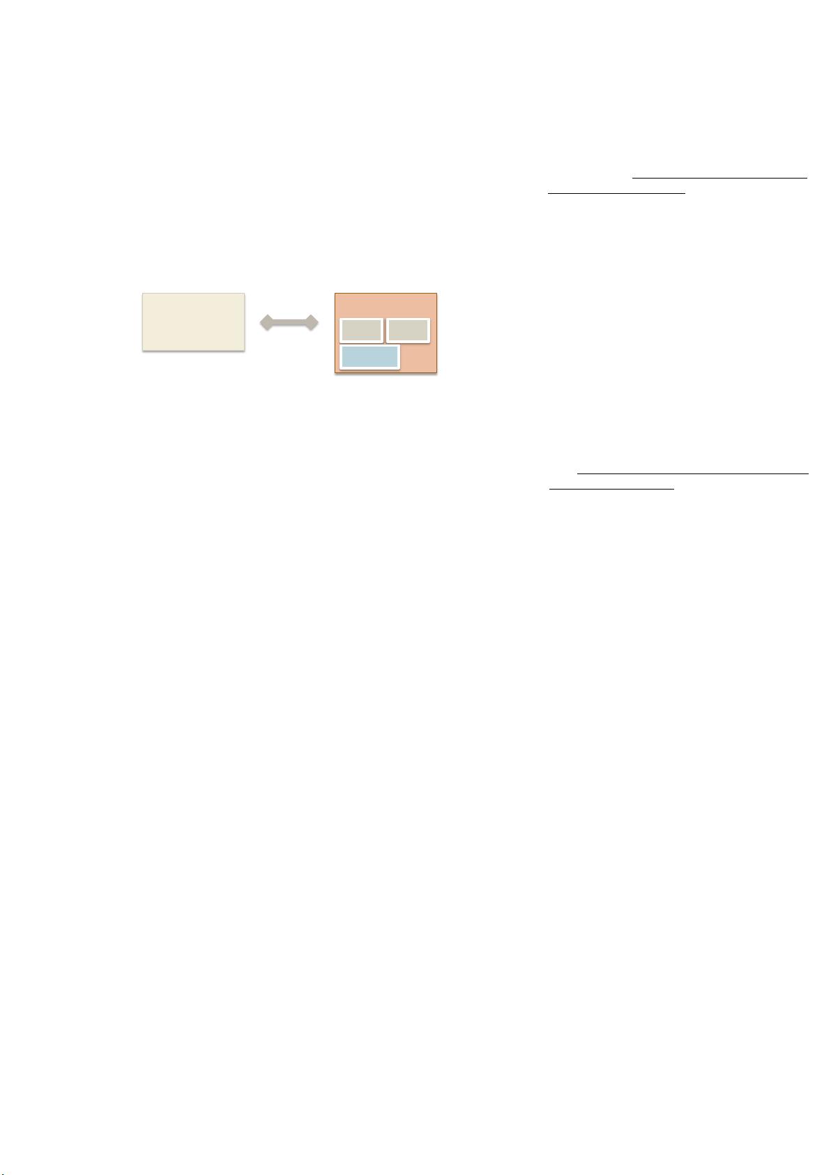
Figure 3: Overview of a co-simulation FMU, note that the solver in this case is within the

FMU.

The FMI standard speciﬁes methods for interacting with a model, providing

variable values and retrieving values. Methods for computing the derivatives,

setting states and time are available for model exchange and for co-simulation,

a method for performing an internal step are available. Furthermore, there are

speciﬁc methods for initialization of a model. The interface is light-weight and

much of the information about the internals are contained in the metadata, i.e.

the XML ﬁle inside the FMU, which needs to be made available.

The standard describes a model exchange FMU with the following underlying

mathematical representation,

˙x = f(t, x, u; p, d) (1a)

y = g(t, x, u; p, d) (1b)

where t is the time, x are the continuous states, u are the inputs, p are the

parameters and d are the discrete variables that are kept constant between

events. Furthermore, y are the outputs. Additionally, the standard supports

diﬀerent types of events which can impact the model behavior. The three events

are:

• State Events

These events are dependent on the state solution proﬁles and thus not

known a prior. The model provides a set of event indicators, z, that the

integrator monitors during the integration process,

DLL XML

FMU

Tool

SolvSolverer

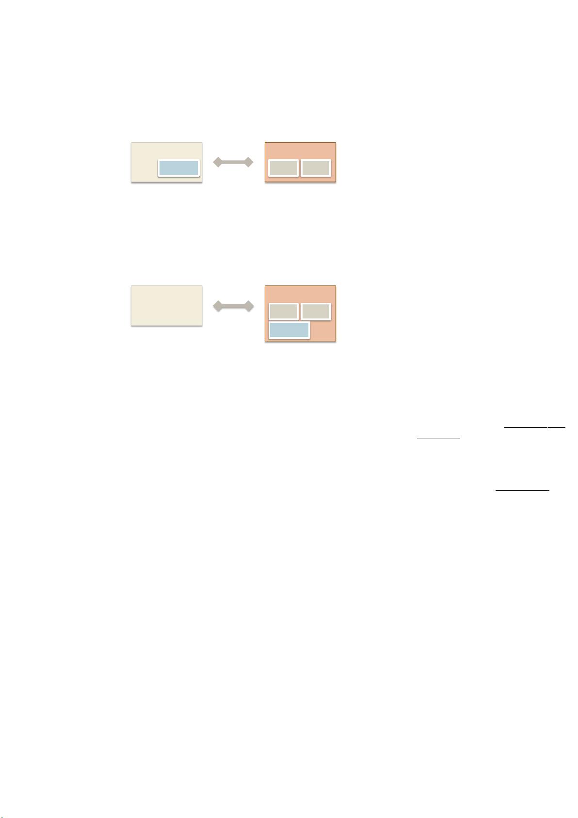
Figure 2: Overview of a model exchange FMU, note that an external solver is required by the

tool in order to solve the model.

DLL XML

FMU

Tool

Solver

FMI标准规定了与模型交互、提供变

量值和检索值的方法。用于计算导数，

设置状态和时间的方法可用于模型交换

和协同仿真，用于执行内部步骤的方法

是可用的。此外，还有用于初始化模型

的特定方法。接口轻量化，大部分内部

信息都包含在元数据中，即FMU内部的

XML文件，这个是必要的。

该标准描述了一个模型交换FMU具有

以下基本数学表示，

其中

是时间，

是连续状态，

u是输入，p

是参数，

是在事件之间保持不变的离散

变量。

此外，

是输出。此外，该标准支

持可能影响模型行为的不同类型的事件。

这三个事件是：

•状态事件

这些事件取决于状态解决配置，因此不

为先验所知。该模型提供了一组事件指

标z，集成商在集成过程中监控这些指

标：

z = h

state

(t, x, u; d, p). (2)

If one of the event indicators, z

, switches domain, there is a state event.

The integrator is then responsible for ﬁnding the time when the event

occurred.

• Time Events

These events on the other hand are known a prior, meaning that for each

simulation segment it is known when the time event occur and thus this

time is set as the simulation end time for that segment. Given a previous

time event, T

pre

(or the initial time, T

), the next time event is computed

using,

= h

time

pre

, x

pre

, u

pre

; d

pre

, p). (3)

An example is that after a certain elapsed time in the integration, a force

is applied on the model.

• Step Events

These last type of events are events that typically do not inﬂuence the

model behavior, instead they are events to ease the numerical integration.

For instance it can be a change of the continuous states in the model as the

current states are no longer appropriate numerically. After each successful

integrator step, T

accepted

, the equation,

step

= h

step

accepted

, x

accepted

, u

accepted

; d

accepted

, p) (4)

is evaluated and if E

step

is True, a step event is triggered.

Further, Equation 1 is valid during continuous simulation and prior to this,

the FMI speciﬁes that the FMU need to be initialized. The simulation and

initialization is separated as to allow a ﬂexible deﬁnition of initial conditions.

An example could be that the initial values for the states are computed using

an initial equation, which is only active during the initialization. The initial

equations are described by,

ˆx

, ˆp = f

init

, ¯x

, u

;

, ¯p), (5)

where ¯x

are states with known initial values,

are the known discrete variables

and ¯p are known parameters. The complete initial states vector is x

= [¯x

, ˆx

and for discrete variables, d

= [

], while the full parameter vector is p =

[¯p, ˆp].

For full details about the mathematical representation, cf. [1] for version 2.0

and [13] for version 1.0.

For co-simulation, the standard rather describes a discrete interface to the

underlying dynamic model, i.e. given the current internal state, input u

and

step size H of the model, return the outputs, y

n+1

, at a time T

+ H = T

n+1

= Φ(H, u

; p), (6)

如果其中一个事件指标z

发生转换，则存在

状态事件。然后，积分器负责查找事件发

生的时间。

·时间事件

另一方面，这些事件是先验已知的，这意

味着对于每个模拟段，已知时间事件何时发

生，因此该时间被设置为该段的模拟结束时

间。给定前一个时间事件T

pre

（或初始时间

），下次使用时计算事件：

一个例子是在积分中经过一定时间后，在模

型上施加力。

·步骤事件

这些最后类型的事件是通常不影响模型行

为的事件，而是它们是简化数值集成的事件。

例如，它可以是模型中连续状态的变化，因为

当前状态不再适合于数字。在每个成功的积分

步长（

accepted

）后

，等式

进行评估，如果Es

tep

为True，则触发步骤事件。

此外，等式

1在连续仿真期间有效，在此之

前，FMI指定需要初始化FMU。仿真和初始化

分离以允许灵活地定义初始条件。一个示例可

以是使用初始方程计算状态的初始值，该初始

方程仅在初始化期间有效。初始方程描述为:

其中x¯0是具有已知初始值的状态，d¯0是已知

的离散变量，而p¯是已知参数。完整的初始状

态向量是x0 = [x¯0，x0]，对于离散变量，d0 =

[d¯0，d0]，而全参数向量是p = [p，p]。

有关数学表示的完整详细信息，请参阅版本

2.0的[1]和版本1.0的[13]。

对于协同仿真，标准描述的是底层动态模型

的离散接口，即给定当前内部状态、输入u

和

模型的步长H，在时间T

+ H =T

N +1

时返回输

出y

+ 1

：

where p are the parameters. The advancement of the states and time are com-

pletely hidden outside of the model and is also not speciﬁed by the standard, cf.

Figure 4. A consequence of this is that, if there are events, these are also handled

internally and are not visible from the outside. There is additionally the restric-

tion that the outputs, y, cannot be evaluated, during simulation, for diﬀerent

inputs, u, without advancing the solution, i.e. performing a step with H > 0.

However, as the advancement is hidden, this allows for specialized solvers to be

Figure 4: A co-simulation FMU and the connection to a tool for simulation. Note that the

solver is inside the FMU.

used for the particular subsystem at hand, which may give an increased per-

formance and a more stable simulation. As in the model exchange case, the

initialization is done separately for co-simulation FMUs. The initialization is

deﬁned by,

ˆp = f

init

, u

; ¯p). (7)

where ¯p are known parameters. The full parameter vector is p = [¯p, ˆp].

For full details about the mathematical representation, cf. [1] for version 2.0

and [14] for version 1.0.

Between version 1.0 and version 2.0 of the standard, changes have been

made. The most signiﬁcant changes are:

• Save/Get state: Methods for retrieving and restoring the internal state

of an FMU have been added.

• Dependency information: Information about which states and inputs

impact the derivatives and the outputs has been added.

• Directional derivatives: Methods for computing the directional deriva-

tives of Equation 1 and Equation 6 has been added.

• Separate initialization: The initialization of an FMU has been sepa-

rated into a state of the FMU instead of a single call to an initialization

method.

• Tunable parameters: Tunable parameters has been added which allow

these types of parameters to be changed at events.

DLL XML

FMU

Tool

Solver

其中p是参数。状态和时间的变化完全隐藏在模

型之外，也没有标准规定，参见图4。这样做的

结果是，如果有事件，这些事件也在内部处理，

并且从外部看不到。另外还有一个限制，即在仿

真期间，如果不推进求解（即H> 0执行一步），

对于不同的输入u，无法评估输出y。

但是，由于隐藏了状态变化，这允许特定子系统

使用专用求解器，可以提高性能和更稳定的仿

真。与模型交换的情况一样，联合仿真FMUs的

初始化是单独进行的。初始化由以下定义：

其中p是已知参数。全参数向量是p = [¯p，p]。

有关数学表示的完整详细信息，请参阅适用于

版本2.0的[1]和适用于版本1.0的[14]。

在标准的1.0版和2.0版之间，已经进行了更改。

最重要的变化是：

· 保存/

获取状态：已添加用于检索和恢复

FMU

内部状态的方法。

·依赖关系信息：添加了有关哪些状态和输

入影响衍生产品和产出的信息。

·方向导数：增加了计算方程1和方程6的方

向导数的方法。

·单独初始化：FMU的初始化已分离为FMU

的状态，而不是单次调用初始化方法。

·可调参数：已添加可调参数，允许在事件

中更改这些类型的参数。

剩余45页未读，继续阅读

wk0svf28

粉丝: 0
资源: 1

会员权益专享

Python工具PyFMI：实现FMI接口的模型仿真

PyFMI:PyFMI是一个软件包，用于为模型交换和协同仿真加载和与功能模型单元（FMU）进行交互，它们是符合功能模型接口（FMI）的已编译动态模型。

Simulink FMI Toolbox

FMI与Matlab联合进行半实物仿真案例（FMI Support in the dSPACE Toolchain.pdf）

Python调用fmu模型

python调用fmu的全部方法

FMU Python

matlab中调用fmu

python程序打包成fmu

python调用fmu的方法

simulink导出fmu模型

xflow fmu计算是什么

FMU的ME（Model Exchange）转换为CS（Co-Simulation）

提供一个python和pyfmi编写的实时调用fmu模型运行的代码案例

simulink中FMU

matlab+fmu

sigfit可以打开FMU模型吗

gtsuite和simulink如何联合仿真

请给出 pyfmi 实时运行 FMU 模型并且实时绘出结果曲线的示例代码：

Isight怎么打开FMU文件呢，请给我具体步骤

matlab FMU

会员权益专享

最新资源