没有合适的资源?快使用搜索试试~ 我知道了~
首页新编《参数估计与逆问题》教材:理论与应用深度解析
"《参数估计与反问题》第二版是一本针对地球物理学、水文学、数学、天体物理学等多个学科的一年级或二年级研究生以及高级本科生的教材,由Rick Aster、Brian Borchers和Clifford H. Thurber合著。该书源于他们在新墨西哥理工学院教授的地质物理逆方法课程,旨在深入讲解参数估计和反问题的基本原理,重点关注不确定性、欠定性、正则化、偏见和分辨率等核心概念。 本书强调理论与实践相结合,通过丰富的例子和MATLAB代码实现,提供了一个配套网站,上面有更多示例和练习的额外材料。读者可以在课程中遇到各种应用和理论问题的练习,包括但不限于数据处理、模型简化和解决实际问题。书中内容广泛,但考虑到篇幅限制和目标读者的知识背景,一些高级主题如逆散射问题、地震散射成像、小波分析、数据同化、模拟退火和期望最大化方法未做详述,这些内容适合对数学基础更扎实的读者进一步研究。 阅读本书的前提是具备大学水平的微积分、微分方程、线性代数、概率论和统计学基础知识。在课程初期,作者通常会回顾这些基础知识,确保学生能跟上教学进度。此外,每章末尾的“注释和进一步阅读”部分为读者提供了深入探讨特定主题的引导,并适当引用了领域的研究成果。 作为一本入门级教材,虽然未能深入探讨所有细节,但它为广大学生和专业人士提供了一个理解物理模型从数据中估计这一通用问题的基础框架。版权方面,该书受到Elsevier公司的保护,未经许可不得任何形式复制或传输。对于版权政策和获取更多许可信息,读者可访问Elsevier的官方网站。"
资源详情
资源推荐
To protect the rights of the author(s) and publisher we inform you that this PDF is an uncorrected proof for internal business use only by the author(s), editor(s),
reviewer(s), Elsevier and typesetter diacriTech. It is not allowed to publish this proof online or in print. This proof copy is the copyright property of the publisher
and is confidential until formal publication.
“Aster Ch01-9780123850485” — 2011/11/8 — page 11 — #11
1.3. Examples of Inverse Problems 11
either require specific strategies or, more commonly, can by solved by iterative methods
that may rely on local linearization.
•
Example 1.6
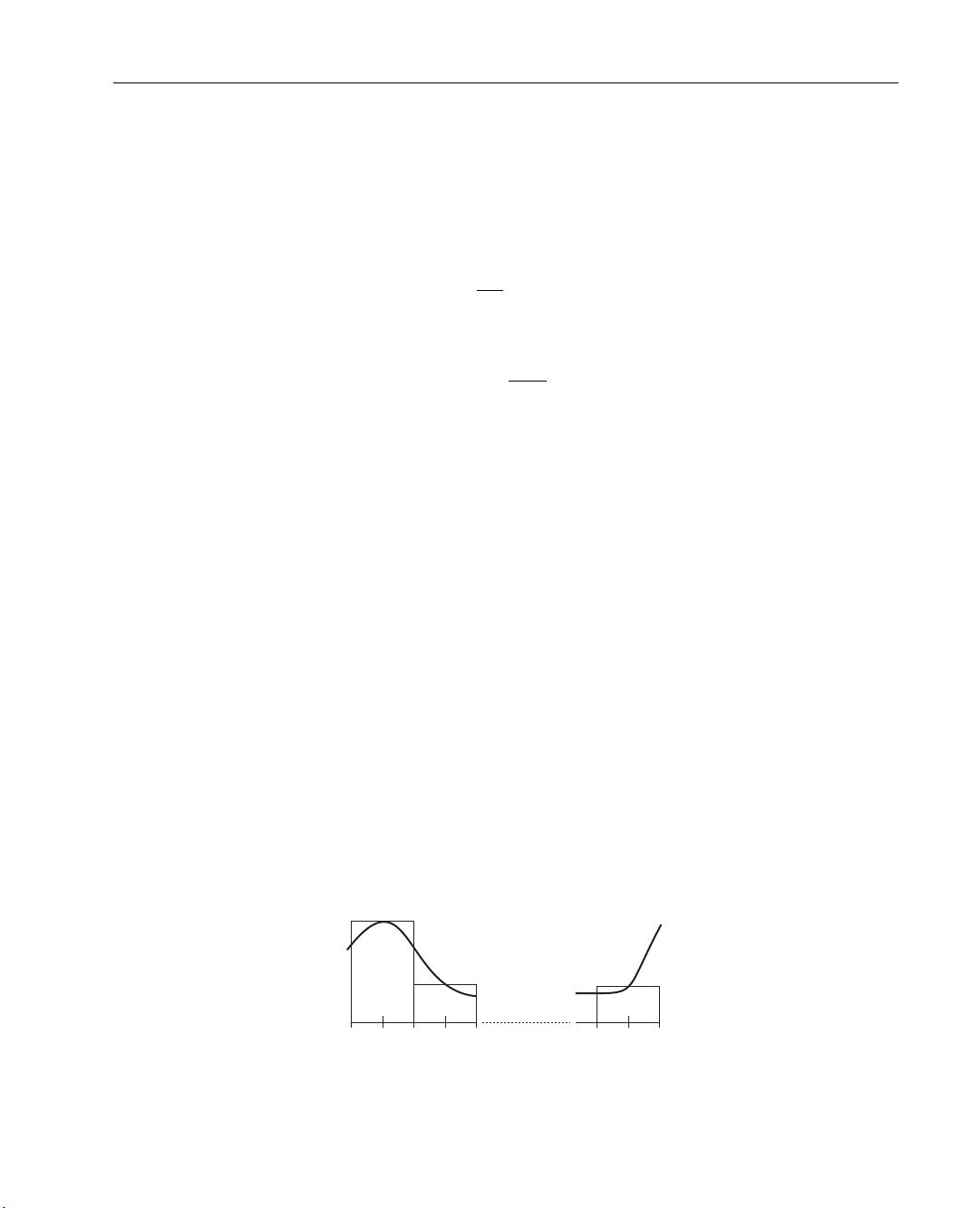
A classic pedagogical inverse problem is an experiment in which an angular distribution
of illumination passes through a thin slit and produces a diffraction pattern, for which
the intensity is observed (Figure 1.6; [141]).
The data, d (s), are measurements of diffracted light intensity as a function of the
outgoing angle −π/2 ≤ s ≤ π/2. Our goal is to find the intensity of the incident light
on the slit, m(θ), as a function of the incoming angle −π/2 ≤ θ ≤ π/2.
The forward problem relating d and m can be expressed as the linear mathematical
model,
d(s) =
π/2
Z
−π/2
(cos(s) +cos(θ ))
2
sin(π(sin(s) +sin(θ)))
π(sin(s) +sin(θ))
2
m(θ)dθ . (1.26)
•
Example 1.7
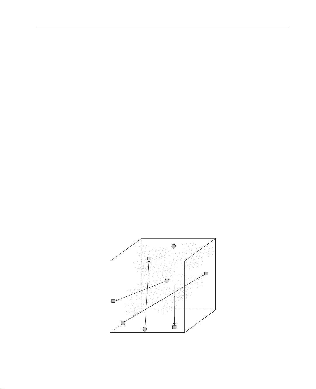
Consider the problem of recovering the history of groundwater pollution at a source
site from later measurements of the contamination at downstream wells to which the
contaminant plume has been transported by advection and diffusion (Figure 1.7). This
Slit
d(s)
m(θ)
θ
s
Figure 1.6 The Shaw diffraction intensity problem (1.26).
To protect the rights of the author(s) and publisher we inform you that this PDF is an uncorrected proof for internal business use only by the author(s), editor(s),
reviewer(s), Elsevier and typesetter diacriTech. It is not allowed to publish this proof online or in print. This proof copy is the copyright property of the publisher
and is confidential until formal publication.
“Aster Ch01-9780123850485” — 2011/11/8 — page 12 — #12
12 Chapter 1 Introduction
0
x
Flow
Figure 1.7 The contaminant plume source history reconstruction problem.
“source history reconstruction problem” has been considered by a number of authors
[117, 144, 145].
The mathematical model for contaminant transport is an advection–diffusion
equation
∂C
∂t
= D
∂
2
C
∂x
2
−v
∂C
∂x
(1.27)
C(0, t) = C
in
(t)
C(x, t) → 0 as x → ∞
where D is the diffusion coefficient and v is the velocity of groundwater flow. The
solution to (1.27) at time T is the convolution
C(x, T ) =
T
Z
0
C
in
(t)f (x, T −t)dt, (1.28)
where C
in
(t) is the time history of contaminant injection at x = 0, and the kernel is
f (x, T −t) =
x
2
p
πD(T −t)
3
e
−
[
x−v(T−t)
]
2
4D(T−t)
. (1.29)
•
Example 1.8
An important and instructive inverse problem is tomography, from the Greek roots
tomos, “to section” or “to cut” (the ancient concept of an atom was that of an irreducible,
uncuttable object) and graphein, “to write.” Tomography is the general technique of
determining models that are consistent with path-integrated properties such as attenu-
ation (e.g., X-ray, radar, muon, seismic), travel time (e.g., electromagnetic, seismic, or
To protect the rights of the author(s) and publisher we inform you that this PDF is an uncorrected proof for internal business use only by the author(s), editor(s),
reviewer(s), Elsevier and typesetter diacriTech. It is not allowed to publish this proof online or in print. This proof copy is the copyright property of the publisher
and is confidential until formal publication.
“Aster Ch01-9780123850485” — 2011/11/8 — page 13 — #13
1.3. Examples of Inverse Problems 13
acoustic), or source intensity (e.g., positron emission). Here, we will use examples from
seismic tomography. Although tomography problems originally involved determining
models that were two-dimensional slices of three-dimensional objects, the term is now
commonly used in situations where the model is two- or three-dimensional. Tomog-
raphy has many applications in medicine, engineering, acoustics, and Earth science.
One important geophysical example is cross-well tomography, where seismic sources
are installed in a borehole, and the signals are received by sensors in another borehole.
Another example is joint earthquake location/velocity structure inversion carried out
on scales ranging from a fraction of a cubic kilometer to global [158, 159, 160].
The physical model for tomography in its most basic form (Figure 1.8) assumes that
geometric ray theory (essentially the high-frequency limiting case of the wave equation)
is valid, so that wave energy traveling between a source and receiver can be considered to
be propagating along infinitesimally narrow ray paths. The density of ray path coverage
in a tomographic problem may vary significantly throughout a section or volume, and
provide much better constraints on physical properties in densely sampled regions than
in sparsely sampled ones.
In seismic tomography, if the slowness at a point x is s(x), and the ray path ` is
known, then the travel time for seismic energy transiting along that ray path is given by
the line integral along `
t =
Z
`
s(x(l))dl. (1.30)
Receivers
Sources
Unknown
internal
structure
Figure 1.8 Conceptual depiction of ray path tomography. Sources and receivers may, in general, be
either at the edges or within the volume, and ray paths may be either straight, as depicted, or curved.
To protect the rights of the author(s) and publisher we inform you that this PDF is an uncorrected proof for internal business use only by the author(s), editor(s),
reviewer(s), Elsevier and typesetter diacriTech. It is not allowed to publish this proof online or in print. This proof copy is the copyright property of the publisher
and is confidential until formal publication.
“Aster Ch01-9780123850485” — 2011/11/8 — page 14 — #14
14 Chapter 1 Introduction
Note that (1.30) is just a higher-dimensional generalization of (1.21), the forward prob-
lem for the vertical seismic profiling example. In general, seismic ray paths will be
bent due to refraction and/or reflection. In cases where such effects are negligible, ray
paths can be usefully approximated as straight lines (e.g., as depicted in Figure 1.8),
and the forward and inverse problems can be cast in a linear form. However, if the ray
paths are significantly bent by slowness variations, the resulting inverse problem will be
nonlinear.
1.4. DISCRETIZING INTEGRAL EQUATIONS
Consider problems of the form
d(x) =
b
Z
a
g(x, ξ)m(ξ)dξ . (1.31)
Here d(x) is a known function, typically representing observed data. The kernel g(x, ξ )
is considered to be given, and encodes the physics relating an unknown model m(x)
to observed data d(s). The interval [a, b] may be finite or infinite. The function d(x)
might in theory be known over an entire interval, but in practice we will only have
measurements of d(x) at a finite set of points.
We wish to solve for m(x). This type of linear equation is called a Fredholm inte-
gral equation of the first kind, or IFK. A surprisingly large number of inverse prob-
lems, including all of the examples from the previous section, can be written as IFKs.
Unfortunately, IFKs have properties that can make them very challenging to solve.
To obtain useful numerical solutions to IFKs, we will frequently discretize them into
forms that are tractably solvable using the methods of linear algebra. We first assume
that d(x) is known at a finite number of points x
1
, x
2
, . . . , x
m
. We can then write the
forward problem as
d
i
= d(x
i
) =
b
Z
a
g(x
i
, ξ )m(ξ )dξ i = 1, 2, . . . , m (1.32)
or as
d
i
=
b
Z
a
g
i
(x)m(x)dx i = 1, 2, . . . , m, (1.33)
where g
i
(x) = g(x
i
, ξ ). The functions g
i
(t) are referred to as representers or data
kernels.
To protect the rights of the author(s) and publisher we inform you that this PDF is an uncorrected proof for internal business use only by the author(s), editor(s),
reviewer(s), Elsevier and typesetter diacriTech. It is not allowed to publish this proof online or in print. This proof copy is the copyright property of the publisher
and is confidential until formal publication.
“Aster Ch01-9780123850485” — 2011/11/8 — page 15 — #15
1.4. Discretizing Integral Equations 15
Here, we will apply a quadrature rule to approximate (1.33) numerically. Note
that, although quadrature methods are applied in this section to linear integral equations,
they also have utility in the discretization of nonlinear problems. The simplest quadrature
approach is the midpoint rule, where we divide the interval [a, b] into n subintervals,
and pick points x
1
, x
2
, . . . , x
n
in the middle of each interval. The points are given by
x
j
= a +
1x
2
+(j −1)1x (1.34)
where
1x =
b −a
n
. (1.35)
The integral (1.33) is then approximated by (Figure 1.9):
d
i
=
b
Z
a
g
i
(x)m(x)dx ≈
n
X
j=1
g
i
(x
j
)m(x
j
)1x, i = 1, 2, . . . , m. (1.36)
If we let
G
i,j
= g
i
(x
j
)1x
i = 1, 2, . . . , m
j = 1, 2, . . . , n
(1.37)
and
m
j
= m(x
j
) j = 1, 2, . . . , n, (1.38)
then we obtain a linear system of equations Gm = d.
The approach of using the midpoint rule to approximate the integral is known as
simple collocation. Of course, there are also more sophisticated quadrature rules for
numerically approximating integrals (e.g., the trapezoidal rule, or Simpson’s rule). In
each case, we end up with an m by n linear system of equations, but the formulas for
evaluating the elements of G will be different.
a x
1
x
2
x
n
b
Figure 1.9 Grid for the midpoint rule.
剩余359页未读,继续阅读
yuankanxue
- 粉丝: 0
- 资源: 2
上传资源 快速赚钱
- 我的内容管理 收起
- 我的资源 快来上传第一个资源
- 我的收益 登录查看自己的收益
- 我的积分 登录查看自己的积分
- 我的C币 登录后查看C币余额
- 我的收藏
- 我的下载
- 下载帮助
会员权益专享
最新资源
- 京瓷TASKalfa系列维修手册:安全与操作指南
- 小波变换在视频压缩中的应用
- Microsoft OfficeXP详解:WordXP、ExcelXP和PowerPointXP
- 雀巢在线媒介投放策划:门户网站与广告效果分析
- 用友NC-V56供应链功能升级详解(84页)
- 计算机病毒与防御策略探索
- 企业网NAT技术实践:2022年部署互联网出口策略
- 软件测试面试必备:概念、原则与常见问题解析
- 2022年Windows IIS服务器内外网配置详解与Serv-U FTP服务器安装
- 中国联通:企业级ICT转型与创新实践
- C#图形图像编程深入解析:GDI+与多媒体应用
- Xilinx AXI Interconnect v2.1用户指南
- DIY编程电缆全攻略:接口类型与自制指南
- 电脑维护与硬盘数据恢复指南
- 计算机网络技术专业剖析:人才培养与改革
- 量化多因子指数增强策略:微观视角的实证分析
资源上传下载、课程学习等过程中有任何疑问或建议,欢迎提出宝贵意见哦~我们会及时处理!
点击此处反馈
安全验证
文档复制为VIP权益,开通VIP直接复制
信息提交成功