没有合适的资源?快使用搜索试试~ 我知道了~
首页HMM算法,隐马尔可夫算法
HMM算法,隐马尔可夫算法
![](https://csdnimg.cn/release/wenkucmsfe/public/img/star.98a08eaa.png)
This chapter is roughly divided into two sections: Hidden Markov Models followed by Maximum Entropy Markov Models. Our discussion of the Hidden Markov Model extends what we said about HMM part-of-speech tagging. We begin in the next section by introducing the Markov Chain, then give a detailed overview of HMMs and the forward and Viterbi algorithms with more formalization, and finally introduce the important EM algorithm for unsupervised (or semi-supervised) learning of a Hidden Markov model.
资源详情
资源推荐
![](https://csdnimg.cn/release/download_crawler_static/3814447/bg1.jpg)
DRAFT
Speech and Language Processing: An introduction to natural language processing,
computational linguistics, and speech recognition. Daniel Jurafsky & James H. Martin.
Copyright
c
2006, All rights reserved. Draft of February 21, 2007. Do not cite
without permission.
6
HIDDEN MARKOV AND
MAXIMUM ENTROPY
MODELS
Numquam ponenda est pluralitas sine necessitat
‘Plurality should never be proposed unless needed’
William of Occam
Tatyana was her name... I own it,
self-willed it may be just the same;
but it’s the first time you’ll have known it,
a novel graced with such a name
Pushkin, Eugene Onegin
In this chapter we introduce two important classes of statistical models for pro-
cessing text and speech, the Hidden Markov Model (HMM) and the Maximum En-
tropy model (MaxEnt), particularly a variant of MaxEnt called the Maximum En-
tropy Markov Model (MEMM). All of these are machine learning models. We have
already touched on some aspects of machine learning; indeed we briefly introduced the
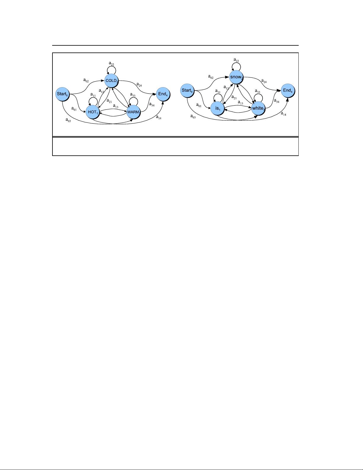
Hidden Markov Model in the previous chapter, and we have introduced the N-gram
model in the chapter before. In this chapter we give a more complete and formal intro-
duction to these two important models.
HMMs and MEMMs are both sequence classifiers. A sequence classifier or
SEQUENCE
CLASSIFIERS
sequence labeler is a model whose job is to assign some label or class to each unit in a
sequence. The finite-state transducer we studied in Ch. 3 is a kind of non-probabilistic
sequence classifier, for example transducing from sequences of words to sequences of
morphemes. The HMM and MEMM extend this notion by being probabilistic sequence
classifiers; given a sequence of units (words, letters, morphemes, sentences, whatever)
their job is to compute a probability distribution over possible labels and choose the
best label sequence.
We have already seen one important sequence classification task: part-of-speech
tagging, where each word in a sequence has to be assigned a part-of-speech tag. Sequence-
labeling tasks come up throughout speech and language processing, a fact that isn’t too
surprising if we consider that language consists of sequences at many representational
![](https://csdnimg.cn/release/download_crawler_static/3814447/bg2.jpg)
DRAFT
2 Chapter 6. Hidden Markov and Maximum Entropy Models
levels. Besides part-of-speech tagging, in this book we will see the application of
these sequence models to tasks like speech recognition (Ch. 9), sentence segmentation
and grapheme-to-phoneme conversion (Ch. 8), partial parsing/chunking (Ch. 12), and
named entity recognition and information extraction (Ch. 17).
This chapter is roughly divided into two sections: Hidden Markov Models fol-
lowed by Maximum Entropy Markov Models. Our discussion of the Hidden Markov
Model extends what we said about HMM part-of-speech tagging. We begin in the next
section by introducing the Markov Chain, then give a detailed overview of HMMs and
the forward and Viterbi algorithms with more formalization, and finally introduce the
important EM algorithm for unsupervised (or semi-supervised) learning of a Hidden
Markov model.
In the second half of the chapter, we introduce Maximum Entropy Markov Mod-
els gradually, beginning with techniques that may already be familiar to you from statis-
tics: linear regression and logistic regression. We next introduce MaxEnt. MaxEnt by
itself is not a sequence classifier; it is used to assign a class to a single element. The
name Maximum Entropy comes from the idea that the classifier finds the probabilis-
tic model which follows Occam’s Razor in being the simplest (least constrained; has
the maximum entropy) yet still consistent with some specific constraints. The Maxi-
mum Entropy Markov Model is the extension of MaxEnt to the sequence labeling task,
adding components such as the Viterbi algorithm.
Although this chapter introduces MaxEnt, which is a classifier, we will not focus
in general on non-sequential classification. Non-sequential classification will be ad-
dressed in later chapters with the introduction of classifiers like the Gaussian Mixture
Model in (Ch. 9) and the Naive Bayes and decision list classifiers in (Ch. 19).
6.1 MARKOV CHAINS
The Hidden Markov Model is one of the most important machine learning models in
speech and language processing. In order to define it properly, we need to first in-
troduce the Markov chain, sometimes called the observed Markov model. Markov
chains and Hidden Markov Models are both extensions of the finite automata of Ch. 3.
Recall that a finite automaton is defined by a set of states, and a set of transitions be-
tween states that are taken based on the input observations. A weighted finite-state
WEIGHTED
automaton is a simple augmentation of the finite automaton in which each arc is asso-
ciated with a probability, indicating how likely that path is to be taken. The probability
on all the arcs leaving a node must sum to 1.
A Markov chain is a special case of a weighted automaton in which the input
MARKOV CHAIN
sequence uniquely determines which states the automaton will go through. Because
they can’t represent inherently ambiguous problems, a Markov chain is only useful for
assigning probabilities to unambiguous sequences.
Fig. 6.1a shows a Markov chain for assigning a probability to a sequence of
weather events, where the vocabulary consists of HOT, COLD, and RAINY,. Fig. 6.1b
shows another simple example of a Markov chain for assigning a probability to a se-
quence of words w
1
...w
n
. This Markov chain should be familiar; in fact it represents a
![](https://csdnimg.cn/release/download_crawler_static/3814447/bg3.jpg)
DRAFT
Section 6.1. Markov Chains 3
(a) (b)
Figure 6.1 A Markov chain for weather (a) and one for words (b). A Markov chain is specified by the structure,
the transition between states, and the start and end states.
bigram language model. Given the two models in Figure 6.1 we can assign a probabil-
ity to any sequence from our vocabulary. We’ll go over how to do this shortly.
First, let’s be more formal. We’ll view a Markov chain as a kind of probabilis-
tic graphical model; a way of representing probabilistic assumptions in a graph. A
Markov chain is specified by the following components:
Q = q
1
q
2
...q
N
a set of states
A = a
01
a
02
...a
n1
...a
nn
a transition probability matrix A, each a
ij
rep-
resenting the probability of moving from state i
to state j, s.t.
P
n
j= 1
a
ij
= 1 ∀i
q
0
,q
end
a special start and end state which are not asso-
ciated with observations.
Fig. 6.1 shows that we represent the states (including start and end states) as
nodes in the graph, and the transitions as edges between nodes.
A Markov chain embodies an important assumption about these probabilities In
a first-order Markov chain, the probability of a particular state is dependent only on
FIRST-ORDER
the previous state:
Markov Assumption: P(q
i
|q
1
...q
i−1
) = P(q
i
|q
i−1
)(6.1)
Note that because each a
ij
expresses the probability p(q
j
|q
i
), the laws of proba-
bility require that the values of the outgoing arcs from a given state must sum to 1:
n
X
j= 1
a
ij
= 1 ∀i(6.2)
An alternate representation that is sometimes used for Markov chains doesn’t
rely on a start or end state, instead representing the distribution over initial states and
accepting states explicitly:
![](https://csdnimg.cn/release/download_crawler_static/3814447/bg4.jpg)
DRAFT
4 Chapter 6. Hidden Markov and Maximum Entropy Models
π = π
1
,π
2
,...,π
N
an initial probability distribution over states. π
i
is the
probability that the Markov chain will start in state i. Some
states j may have π
j
= 0, meaning that they cannot be initial
states. Also,
P
n
i=1
π
i
= 1
QA = {q
x
,q
y
...} a set QA ⊂ Q of legal accepting states
Thus the probability of state 1 being the first state can be represented either as
a
01
or as π
1
. Note that because each π
i
expresses the probability p(q
i
|START), all the
π probabilities must sum to 1:
n
X
i=1
π
i
= 1(6.3)
(a) (b)
Figure 6.2 Another representation of the same Markov chain for weather shown in Fig. 6.1. Instead of using
a special start state with a
01
transition probabilities, we use the π vector, which represents the distribution over
starting state probabilities. The figure in (b) shows sample probabilities.
Before you go on, use the sample probabilities in Fig. 6.2b to compute the prob-
ability of each of the following sequences:
(6.4) hot hot hot hot
(6.5) cold hot cold hot
What does the difference in these probabilities tell you about a real-world weather
fact encoded in Fig. 6.2b?
6.2 THE HIDDEN MARKOV MODEL
A Markov chain is useful when we need to compute a probability for a sequence of
events that we can observe in the world. In many cases, however, the events we are
![](https://csdnimg.cn/release/download_crawler_static/3814447/bg5.jpg)
DRAFT
Section 6.2. The Hidden Markov Model 5
interested in may not be directly observable in the world. For example for part-of-
speech tagging (Ch. 5) we didn’t observe part of speech tags in the world; we saw
words, and had to infer the correct tags from the word sequence. We call the part-
of-speech tags hidden because they are not observed. We will see the same thing
in speech recognition; we’ll see acoustic events in the world, and have to infer the
presence of ‘hidden’ words that are the underlying causal source of the acoustics. A
Hidden Markov Model (HMM) allows us to talk about both observed events (like
HIDDEN MARKOV
MODEL
words that we see in the input) and hidden events (like part-of-speech tags) that we
think of as causal factors in our probabilistic model.
To exemplify these models, we’ll use a task conceived of by Jason Eisner (2002).
Imagine that you are a climatologist in the year 2799 studying the history of global
warming. You cannot find any records of the weather in Baltimore, Maryland, for the
summer of 2007, but you do find Jason Eisner’s diary, which lists how many ice creams
Jason ate every day that summer. Our goal is to use these observations to estimate the
temperature every day. We’ll simplify this weather task by assuming there are only two
kinds of days: cold (C) and hot (H). So the Eisner task is as follows:
Given a sequence of observations O, each observation an integer corre-
sponding to the number of ice creams eaten on a given day, figure out the
correct ‘hidden’ sequence Q of weather states (H or C) which caused Jason
to eat the ice cream.
Let’s begin by seeing how a Hidden Markov Model differs from a Markov chain.
An HMM is specified by a set of states Q, a set of transition probabilities A, a
HMM
set of observation likelihoods B, a defined start state and end state(s), and a set of
observation symbols O, which is not drawn from the same alphabet as the state set Q:
Let’s begin with a formal definition of a Hidden Markov Model, focusing on how
it differs from a Markov chain. An HMM is specified by the following components:
HMM
Q = q
1
q
2
...q
N
a set of states
A = a
01
a
02
...a
n1
...a
nn
a transition probability matrix A, each a
ij
rep-
resenting the probability of moving from state i
to state j, s.t.
P
n
j= 1
a
ij
= 1 ∀i
O = o
1
o
2
...o
N
a set of observations, each one drawn from a vo-
cabulary V = v
1
,v
2
,...,v
V
.
B = b
i
(o
t
) A set of observation likelihoods:, also called
emission probabilities, each expressing the
probability of an observation o
t
being generated
from a state i.
q
0
,q
end
a special start and end state which are not asso-
ciated with observations.
As we noted for Markov chains, an alternate representation that is sometimes
used for HMMs doesn’t rely on a start or end state, instead representing the distribution
over initial and accepting states explicitly:
剩余41页未读,继续阅读
![pptx](https://img-home.csdnimg.cn/images/20210720083543.png)
![](https://csdnimg.cn/download_wenku/file_type_ask_c1.png)
安全验证
文档复制为VIP权益,开通VIP直接复制
![](https://csdnimg.cn/release/wenkucmsfe/public/img/green-success.6a4acb44.png)