
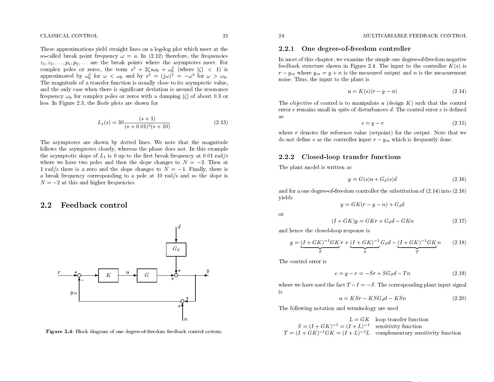
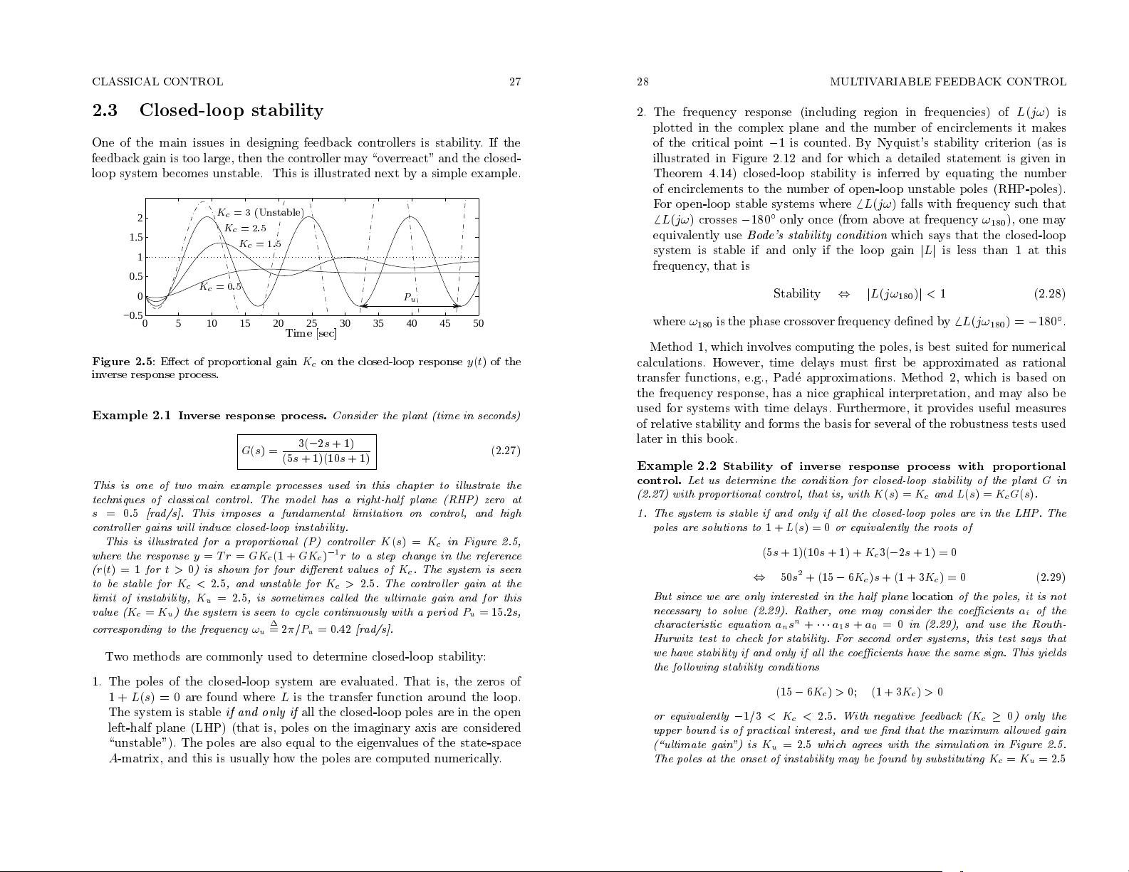
CLASSICAL CONTROL 21
where wehaveused
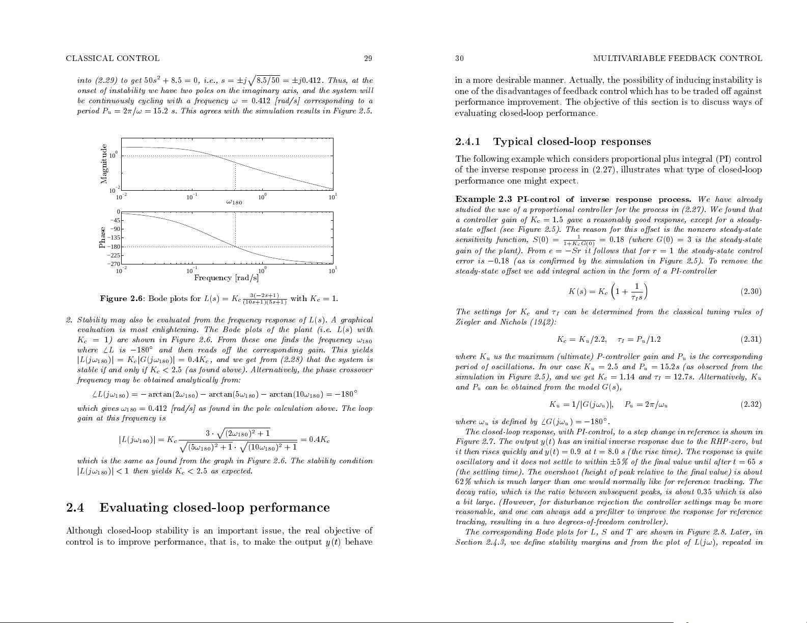
!
as an argument b ecause
y
0
and
depend on frequency,
and in some cases so may
u
0
and
. Note that
u
(
!
) is
not
equal to
u
(
s
)
evaluated at
s
=
!
nor is it equal to
u
(
t
) evaluated at
t
=
!
. Since
G
(
j!
)=
j
G
(
j!
)
j
e
j
6
G
(
j!
)
the sinusoidal resp onse in (2.5) and (2.6) can then
be written on complex form as follows
y
(
!
)
e
j!t
=
G
(
j!
)
u
(
!
)
e
j!t
(2.8)
or because the term
e
j!t
appears on b oth sides
y
(
!
)=
G
(
j!
)
u
(
!
) (2.9)
whichwe refer to as the phasor notation. At each frequency,
u
(
!
),
y
(
!
)and
G
(
j!
) are complex numbers, and the usual rules for multiplying complex
numb ers apply.We will use this phasor notation throughout the bo ok. Thus
whenever we use notation such as
u
(
!
)
(with
!
and not
j!
as an argument),
the reader should interpret this as a (complex) sinusoidal signal,
u
(
!
)
e
j!t
.
(2.9) also applies to MIMO systems where
u
(
!
)and
y
(
!
) are complex vectors
representing the sinusoidal signal in each channel and
G
(
j!
) is a complex
matrix.
Minimum phase systems.
For stable systems which are minimum phase
(no time delays or right-half plane (RHP) zeros) there is a unique relationship
between the gain and phase of the frequency resp onse. This maybequantied
by the Bode gain-phase relationship whichgives the phase of
G
(normalized
1
suchthat
G
(0)
>
0) at a given frequency
!
0
as a function of
j
G
(
j!
)
j
over the
entire frequency range:
6
G
(
j!
0
)=
1
Z
1
;1
d
ln
j
G
(
j!
)
j
d
ln
!
|
{z }
N
(
!
)
ln
!
+
!
0
!
;
!
0
d!
!
(2.10)
The name
minimum phase
refers to the fact that such a system has the
minimum p ossible phase lag for the given magnitude resp onse
j
G
(
j!
)
j
. The
term
N
(
!
) is the slop e of the magnitude in log-variables at frequency
!
.In
particular, the local slop e at frequency
!
0
is
N
(
!
0
)=
d
ln
j
G
(
j!
)
j
d
ln
!
!
=
!
0
(2.11)
The term ln
!
+
!
0
!
;
!
0
in (2.10) is innite at
!
=
!
0
, so it follows that
6
G
(
j!
0
)is
primarily determined by the lo cal slope
N
(
!
0
). Also
R
1
;1
ln
!
+
!
0
!
;
!
0
d!
!
=
2
2
1
The normalization of
G
(
s
) is necessary to handle systems suchas
1
s
+2
and
;
1
s
+2
,which
have equal gain, are stable and minimum phase, but their phases dier by 180
. Systems
with integrators may b e treated by replacing
1
s
by
1
s
+
where
is a small positivenumber.
22 MULTIVARIABLE FEEDBACK CONTROL
which justies the commonly used approximation for stable minimum phase
systems
6
G
(
j!
0
)
2
N
(
!
0
)rad]=90
N
(
!
0
)
The approximation is exact for the system
G
(
s
)=1
=s
n
(where
N
(
!
)=
;
n
),
and it is go o d for stable minimum phase systems except at frequencies close
to those of resonance (complex) p oles or zeros.
RHP-zeros and time delays contribute additional phase lag to a system when
compared to that of a minimum phase system with the same gain (hence the
term
non-minimum phase
system). For example, the system
G
(
s
)=
;
s
+
a
s
+
a
with
a RHP-zero at
s
=
a
has a constant gain of 1, but its phase is
;
2 arctan(
!=a
)
rad] (and not 0 rad] as it would b e for the minimum phase system
G
(
s
)=1
of the same gain). Similarly, the time delay system
e
;
s
has a constant gain
of 1, but its phase is
;
!
rad].
10
−3
10
−2
10
−1
10
0
10
1
10
2
10
3
10
−5
10
0
10
5
0
−2
−1
−2
10
−3
10
−2
10
−1
10
0
10
1
10
2
10
3
−180
−135
−90
−45
0
Magnitude
Frequency rad/s]
Phase
!
1
!
2
!
3
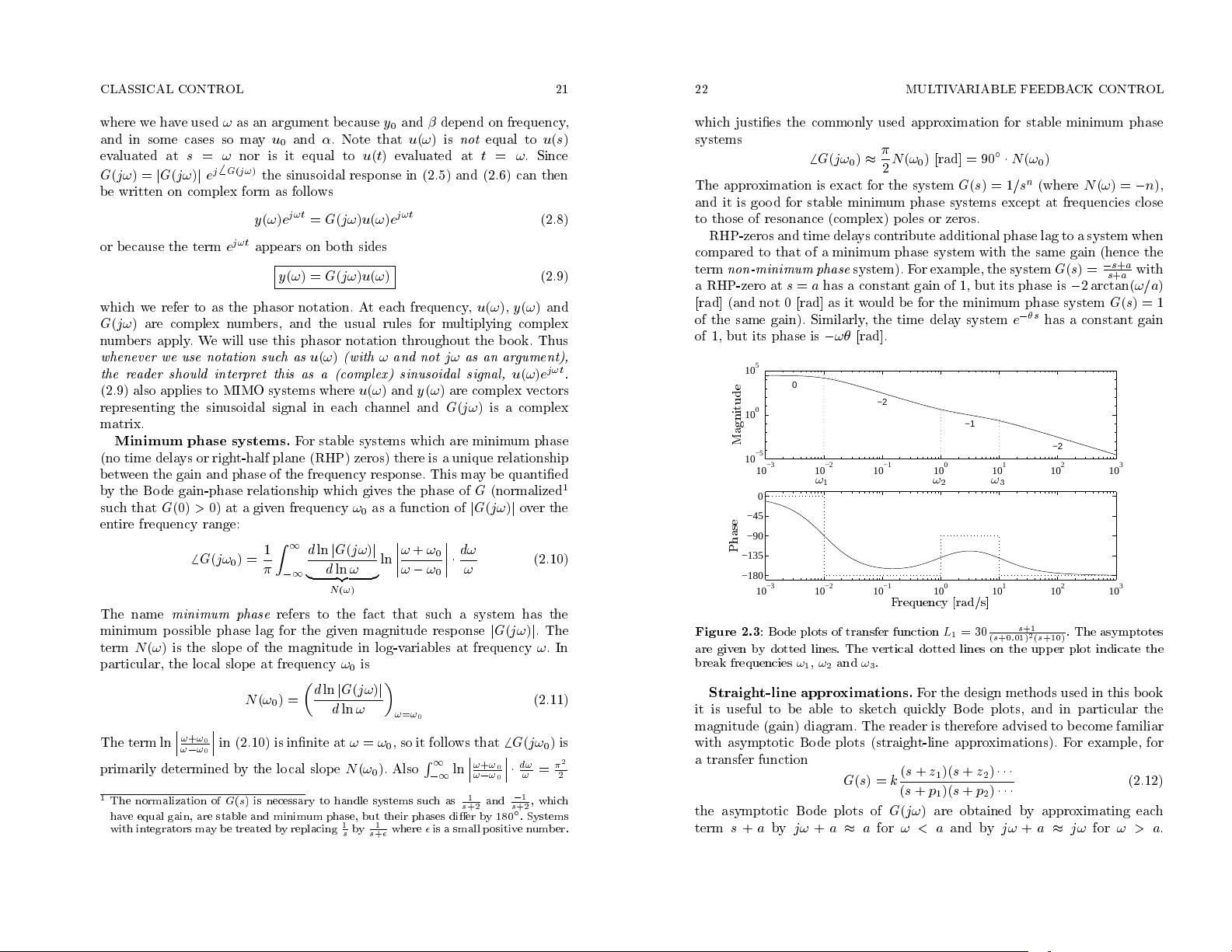
Figure 2.3
: Bode plots of transfer function
L
1
=30
s
+1
(
s
+0
:
01)
2
(
s
+10)
. The asymptotes
are given by dotted lines. The vertical dotted lines on the upp er plot indicate the
break frequencies
!
1
,
!
2
and
!
3
.
Straight-line approximations.
For the design metho ds used in this b o ok
it is useful to be able to sketch quickly Bode plots, and in particular the
magnitude (gain) diagram. The reader is therefore advised to become familiar
with asymptotic Bo de plots (straight-line approximations). For example, for
a transfer function
G
(
s
)=
k
(
s
+
z
1
)(
s
+
z
2
)
(
s
+
p
1
)(
s
+
p
2
)
(2.12)
the asymptotic Bode plots of
G
(
j!
) are obtained by approximating each
term
s
+
a
by
j!
+
a
a
for
! < a
and by
j!
+
a
j!
for
! > a
.
剩余302页未读,继续阅读

fengli_09
- 粉丝: 0
- 资源: 9
 我的内容管理
收起
我的内容管理
收起
- 我的资源
快来上传第一个资源
 我的收益 登录查看自己的收益
 我的积分
登录查看自己的积分
我的积分
登录查看自己的积分
 我的C币
登录后查看C币余额
我的C币
登录后查看C币余额
 我的收藏
我的收藏  我的下载
我的下载  下载帮助
下载帮助

会员权益专享


最新资源
- 构建智慧路灯大数据平台:物联网与节能解决方案
- 智慧开发区建设:探索创新解决方案
- SQL查询实践:员工、商品与销售数据分析
- 2022智慧酒店解决方案:提升服务效率与体验
- 2022年智慧景区信息化整体解决方案:打造数字化旅游新时代
- 2022智慧景区建设:大数据驱动的5A级管理与服务升级
- 2022智慧教育综合方案:迈向2.0时代的创新路径与实施策略
- 2022智慧教育:构建区域教育云,赋能学习新时代
- 2022智慧教室解决方案:融合技术提升教学新时代
- 构建智慧机场:2022年全面信息化解决方案
- 2022智慧机场建设:大数据与物联网引领的生态转型与客户体验升级
- 智慧机场2022安防解决方案:打造高效指挥与全面监控系统
- 2022智慧化工园区一体化管理与运营解决方案
- 2022智慧河长管理系统:科技助力水环境治理
- 伪随机相位编码雷达仿真及FFT增益分析
- 2022智慧管廊建设:工业化与智能化解决方案
资源上传下载、课程学习等过程中有任何疑问或建议,欢迎提出宝贵意见哦~我们会及时处理!
点击此处反馈


