
484 J. Comput. Sci. & Technol., July 2008, Vol.23, No.4
mining pattern-based clusters. For example, the Pear-
son R model
[18]
studies the coherence among a set of
objects, and Pearson R defines the correlation between
two objects X and Y as:
X
i
(X
i
− X)(Y
i
− Y )
s
X
i
(X
i
− X)
2
×
X
i
(Y
i
− Y )
2
where X
i
and Y
i
are the i-th attribute value of X and
Y , and X and Y are the means of all attribute values
in X and Y , respectively. From this formula, we can
see that the Pearson R correlation measures the corre-
lation between two objects with respect to all attribute
values. A large positive value indicates a strong pos-
itive correlation while a large negative value indicates
a strong negative correlation. However, some strong
coherence may only exist on a subset of dimensions.
For example, in collaborative filtering, six movies are
ranked by viewers. The first three are action movies
and the next three are family movies. Two viewers
rank the movies as (8, 7, 9, 2, 2, 3) and (2, 1, 3, 8, 8, 9).
The viewers’ ranking can be grouped into two clusters,
the first three movies in one cluster and the rest in an-
other. It is clear that the two viewers have consistent
bias within each cluster. However, the P earson R cor-
relation of the two viewers is small because globally no
explicit pattern exists.
2.2 Correlations in Subspaces
One way to discover the shifting pattern in Fig.2(a)
using traditional subspace clustering algorithms (such
as CLIQUE) is through data transformation. Given N
attributes, a
1
, . . . , a
N
, we define a derived attribute,
A
ij
= a
i
− a
j
, for every pair of attributes a
i
and
a
j
. Thus, our problem is equivalent to mining sub-
space clusters on the objects with the derived set of
attributes. However, the converted data set will have
N(N −1)/2 dimensions and it becomes intractable even
for a small N because of the curse of dimensionality.
Cheng et al. introduced the bicluster concept
[15]
as
a measure of the coherence of the genes and conditions
in a sub matrix of a DNA array. Let X be the set
of genes and Y the set of conditions. Let I ⊂ X and
J ⊂ Y be subsets of genes and conditions, respectively.
The pair (I, J) specifies a sub matrix A
IJ
with the fol-
lowing mean squared residue score:
H(I, J) =
1
|IkJ|
X
i∈I,j∈J
(d
ij
− d
iJ
− d
Ij
+ d
IJ
)
2
, (1)
where
d
iJ
=
1
|J|
X
j∈J
d
ij
, d
Ij
=
1
|I|
X
i∈I
d
ij
,
d
IJ
=
1
|I||J|
X
i∈I,j∈J
d
ij
are the row and column means and the means in the
submatrix A
IJ
, respectively. A submatrix A
IJ
is called
a δ-bicluster if H(I, J) 6 δ for some δ > 0. A random
algorithm is designed for finding such clusters in a DNA
array.
Yang et al.
[16]
proposed a move-based algorithm to
find biclusters more efficiently. It starts from a random
set of seeds (initial clusters) and iteratively improves
the clustering quality. It avoids the cluster overlapping
problem as multiple clusters are found simultaneously.
However, it still has the outlier problem, and it requires
the number of clusters as an input parameter.
We noticed several limitations of this pioneering
work as follows.
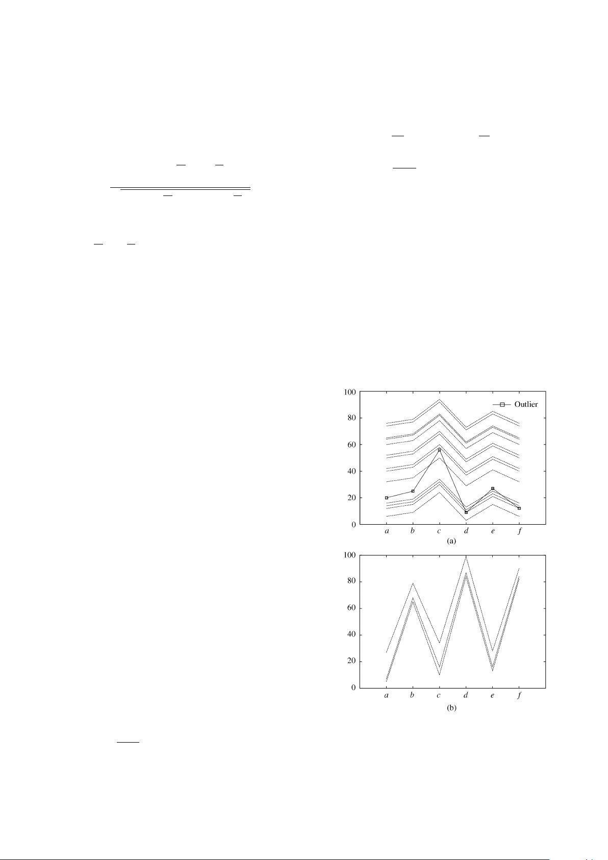
Fig.3. Mean squared residue cannot exclude outliers in a biclus-
ter. (a) Dataset A: Residue 4.238 (without the outlier residue is
0). (b) Dataset B: Residue 5.722.
剩余15页未读,继续阅读

gly20031015
- 粉丝: 0
- 资源: 1
 我的内容管理
展开
我的内容管理
展开


最新资源
- 构建Cadence PSpice仿真模型库教程
- VMware 10.0安装指南:步骤详解与网络、文件共享解决方案
- 中国互联网20周年必读:影响行业的100本经典书籍
- SQL Server 2000 Analysis Services的经典MDX查询示例
- VC6.0 MFC操作Excel教程:亲测Win7下的应用与保存技巧
- 使用Python NetworkX处理网络图
- 科技驱动:计算机控制技术的革新与应用
- MF-1型机器人硬件与robobasic编程详解
- ADC性能指标解析:超越位数、SNR和谐波
- 通用示波器改造为逻辑分析仪:0-1字符显示与电路设计
- C++实现TCP控制台客户端
- SOA架构下ESB在卷烟厂的信息整合与决策支持
- 三维人脸识别:技术进展与应用解析
- 单张人脸图像的眼镜边框自动去除方法
- C语言绘制图形:余弦曲线与正弦函数示例
- Matlab 文件操作入门:fopen、fclose、fprintf、fscanf 等函数使用详解
资源上传下载、课程学习等过程中有任何疑问或建议,欢迎提出宝贵意见哦~我们会及时处理!
点击此处反馈


