Sensors 2017, 17, 818 4 of 16
traffic information on each road segment can be estimated and integrated further into a time-space
matrix that serves as a time-space image.
In the time dimension, time usually ranges from the beginning to the end of a day, and time intervals,
which are usually 10 s to 5 min, depend on the sampling resolution of the GPS devices. Generally,
narrow intervals, for example 10 s, are meaningless for traffic prediction. Thus, if the sampling
resolution is high, these data may be aggregated to obtain wider intervals, such as several minutes.
In the space dimension, the selected trajectory is viewed as a sequence of dots with inner states,
including vehicle position, average speed, etc. This sequence of dots can be ordered simply and
linearly fitted into the y-axis, but may result in a high dimension and uninformative issues, because
the sequences of dots are redundant and a large number of regions in this sequence are stable and
lack variety. Therefore, to make the y-axis both compact and informative, the dots are grouped into
sections, each representing a similar traffic state. The sections are then ordered spatially with reference
to a predefined start point of a road, and then fitted into the y-axis.
Finally, a time-space matrix can be constructed using time and space dimension information.
Mathematically, we denote the time-space matrix by:
M =
m
11
, m
12
, · · · , m
1N
m
21
, m
22
, · · · , m
2N
.
.
.
.
.
. · · ·
.
.
.
m
Q1
, m
Q2
, · · · , m
QN
(1)
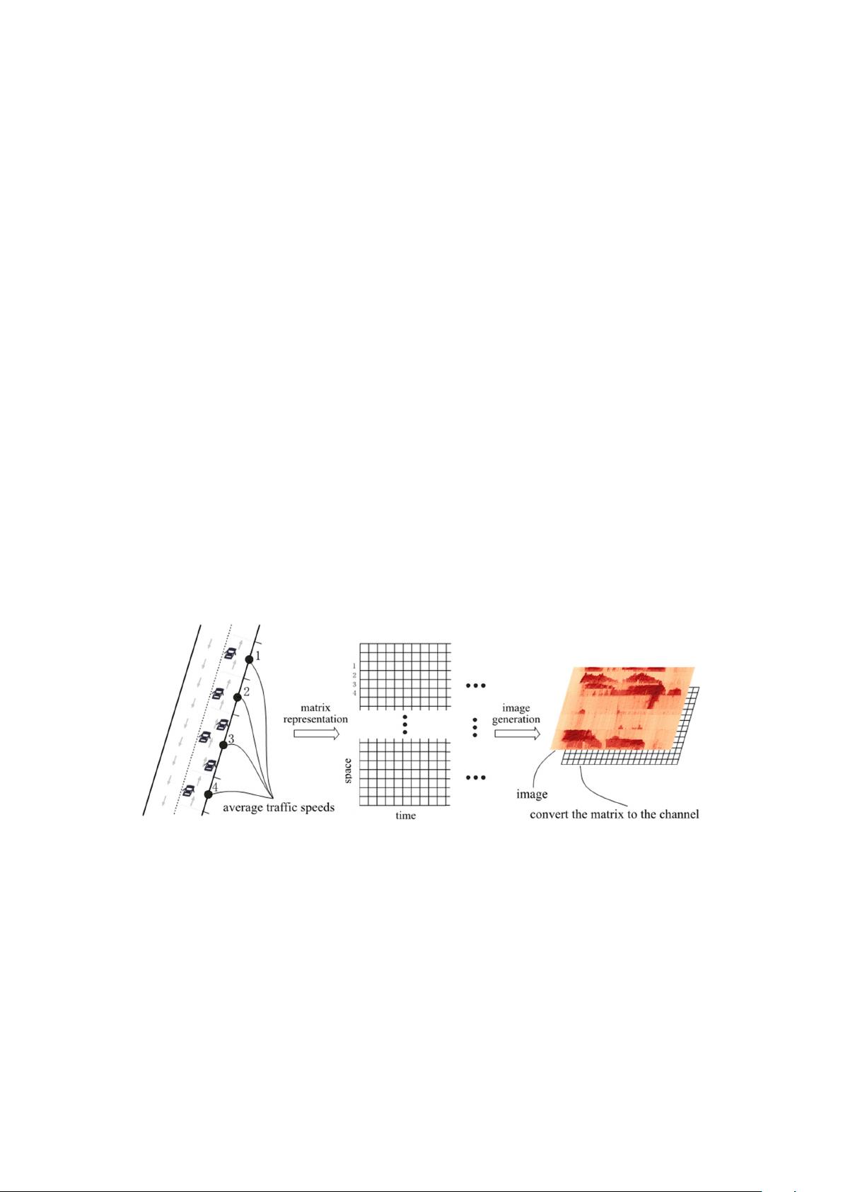
where N is the length of time intervals, Q is the length of road sections; the ith column vector of M is
the traffic speed of the transportation network at time i; and pixel m
ij
is the average traffic speed on
section i at time j. Matrix M forms a channel of the image. Figure 1 illustrates the relations among raw
averaged floating car speeds, time-space matrix, and the final image.
Sensors 2017, 17, 818 4 of 16
traffic information on each road segment can be estimated and integrated further into a time-space
matrix that serves as a time-space image.
In the time dimension, time usually ranges from the beginning to the end of a day, and time
intervals, which are usually 10 s to 5 min, depend on the sampling resolution of the GPS devices.
Generally, narrow intervals, for example 10 s, are meaningless for traffic prediction. Thus, if the
sampling resolution is high, these data may be aggregated to obtain wider intervals, such as several
minutes.
In the space dimension, the selected trajectory is viewed as a sequence of dots with inner states,
including vehicle position, average speed, etc. This sequence of dots can be ordered simply and
linearly fitted into the y-axis, but may result in a high dimension and uninformative issues, because
the sequences of dots are redundant and a large number of regions in this sequence are stable and
lack variety. Therefore, to make the y-axis both compact and informative, the dots are grouped into
sections, each representing a similar traffic state. The sections are then ordered spatially with
reference to a predefined start point of a road, and then fitted into the y-axis.
Finally, a time-space matrix can be constructed using time and space dimension information.
Mathematically, we denote the time-space matrix by:
11 12 1
21 22 2
12
,,,
,,,
,,,
N
N
QQ QN
mm m
mm m
M
mm m
(1)
where N is the length of time intervals, Q is the length of road sections; the ith column vector of M is
the traffic speed of the transportation network at time i; and pixel m
ij
is the average traffic speed on
section i at time j. Matrix M forms a channel of the image. Figure 1 illustrates the relations among raw
averaged floating car speeds, time-space matrix, and the final image.
Figure 1. An illustration of the traffic-to-image conversion on a network.
2.2. CNN for Network Traffic Prediction
2.2.1. CNN Characteristics
The CNN has exhibited a significant learning ability in image understanding because of its
unique method of extracting critical features from images. Compared to other deep learning
architectures, two salient characteristics contribute to the uniqueness of CNN, namely, (a) locally-
connected layers, which means output neurons in the layers are connected only to their local nearby
input neurons, rather than the entire input neurons in fully-connected layers. These layers can extract
features from an image effectively, because every layer attempts to retrieve a different feature
regarding the prediction problem [31]; and (b) a pooling mechanism, which largely reduces the
number of parameters required to train the CNN while guaranteeing that the most important features
are preserved.
Figure 1. An illustration of the traffic-to-image conversion on a network.
2.2. CNN for Network Traffic Prediction
2.2.1. CNN Characteristics
The CNN has exhibited a significant learning ability in image understanding because of its unique
method of extracting critical features from images. Compared to other deep learning architectures,
two salient characteristics contribute to the uniqueness of CNN, namely, (a) locally-connected layers,
which means output neurons in the layers are connected only to their local nearby input neurons,
rather than the entire input neurons in fully-connected layers. These layers can extract features
from an image effectively, because every layer attempts to retrieve a different feature regarding the
prediction problem [
31
]; and (b) a pooling mechanism, which largely reduces the number of parameters
required to train the CNN while guaranteeing that the most important features are preserved.


