3.3 Boundary Blur Estimation
If we merely use per-segment affine reconstruction, the
reconstructed image has artificial boundaries, and the
original boundaries would be artificially sharpened. To
avoid that, we estimate the blur from the original image in
the following way. For each hypothesized blur b from
b
min
ð¼ 0Þ to b
max
ð¼ 2:5Þ in steps of bð¼ 0:25Þ, we compute
the blurred image f
blur
ðv; bÞ¼fðvÞGðu; bÞ, where Gðu; bÞ
is a Gaussian kernel with sigma b. We then compute the
error image I
err
such that I
err
ðv; bÞ¼kIðvÞf
blur
ðv; bÞk
2
.
We dilate each boundary curve C
ij
five times into regions
i
and
j
to obtain a mask
ij
. The best blur b
ij
for C
ij
corresponds to the minimum aggregate error I
err
ðv; bÞ over
ij
or b
ij
¼ arg min
b
P
v2
ij
I
err
ðv; bÞ.
To reinstate the blur in the transition region
ij
,we
simply replace fðvÞ with f
blur
ðv; b
ij
Þ. Note that this assumes
that the amount of blur in
i
and
j
is the same, which is
strictly not true in general. However, we found that this
approximation generates satisfactory results. After this
process is done for every pair of region s, we obtain
boundary blurred piecewise affine reconstruction f
blur
ðvÞ.
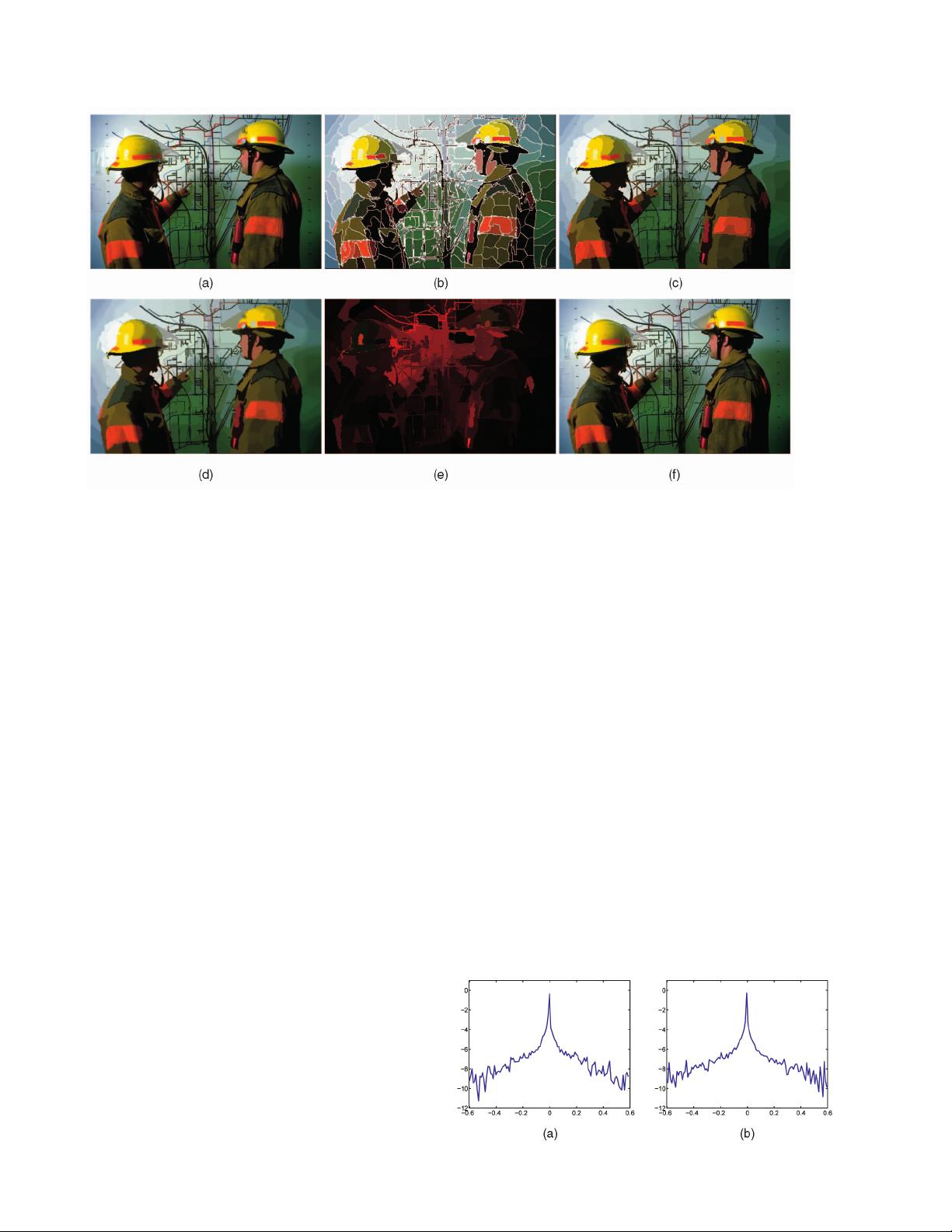
The piecewise smooth image model is illustrated in
Figs. 1a, 1b, 1c, and 1d. The example image (Fig. 1a) taken
from Berkeley image segmentation database [32] is parti-
tioned to piecewise smooth regions (Fig. 1b) by the segmenta-
tion algorithm. The per-segment affine reconstruction is
shown in Fig. 1c, where we can see artificial boundaries
between regions and the true boundaries are sharpened. After
blur estimation and reinstatement in Fig. 1d, the boundaries
become much smoother.
3.4 Important Properties of the Piecewise Smooth
Image Model
There are three important properties of our piecewise
smooth image model that led us to choose it as the model
for both noise estimation and removal. They are
1. the piecewise smooth image model is consistent with
a sparse image prior;
2. the color distribution per each segment can be well
approximated by a line segment, due to the physics
of image formation [26], [24], [20]; and
3. the standard deviation of residual per each segment
is the upper bound of the noise level in that segment.
The last property follows from (3). For the first two
properties, we again use the example image in Fig. 1a to
examine them. For the reconstructed image (Fig. 1d), we
compute the log histograms of the horizontal and vertical
derivatives and plotted them in Fig. 2. The long tails clearly
show that the piecewise smooth reconstruction match the
high-kurtosis statistics of natural images [33]. This image
model also shares some similarity with the so-called dead
leaves model [29].
For the second property, we compute the eigenvalues and
eigenvectors of the RGB values f IðvÞg in each region. The
eigenvalues are sorted in descending order and displayed in
Fig. 1e. Obviously, the red channel accounts for the majority
of the RGB channels, a fact that proves the first eigenvalue of
each segment is significantly larger than the second eigenva-
lue. Therefore, when we project the pixel values onto the first
302 IEEE TRANSACTIONS ON PATTERN ANALYSIS AND MACHINE INTELLIGENCE, VOL. 30, NO. 2, FEBRUARY 2008
Fig. 1. Illustration of piecewise smooth image model. (a) Original image. (b) Segmentation. (c) Per-segment affine reconstruction. (d) Affine
reconstruction plus boundary blur. (e) The sorted eigenvalues in each segment. (f) RGB values projected onto the largest eigenvector.
Fig. 2. The log histograms of the (a) horizontal and (b) vertical derivative
filter responses of the reconstruction in Fig. 1d.


