figure N = fs*Tp; freq = linspace(-B/2, B/2, N); plot(freq/1e6, fftshift(abs(fft(Sig_rec)))); xlabel('频率/MHz');ylabel('幅度'); grid on; hold on; plot(freq/1e6, fftshift(abs(fft(Sig_jam))),'r'); xlim([-1 4]); legend('回波信号','干扰信号');把回波信号去掉不显示回波信号图像

时间: 2023-07-15 17:12:22 浏览: 31
如果要去掉回波信号的图像,可以在绘制回波信号的代码行上加上一个注释符号 %,使其变成注释掉的代码行。具体地,修改后的代码如下: ```matlab figure N = fs*Tp; freq = linspace(-B/2, B/2, N); plot(freq/1e6, fftshift(abs(fft(Sig_rec)))); % 注释掉回波信号的绘图语句 xlabel('频率/MHz');ylabel('幅度'); grid on; hold on; plot(freq/1e6, fftshift(abs(fft(Sig_jam))),'r'); xlim([-1 4]); legend('干扰信号'); % 修改图例,只显示干扰信号 ``` 这样修改后,只会绘制干扰信号的图像,并且图例也只显示干扰信号。
相关问题

N = fs*Tp; freq = linspace(-B/2, B/2, N); % plot(freq/1e6, fftshift(abs(fft(Sig_rec)))); % xlabel('频率/MHz');ylabel('幅度'); % grid on; hold on; % plot(freq/1e6, fftshift(abs(fft(Sig_jam))),'r'); % xlim([-1 4]); % legend('回波信号','干扰信号');

这段代码是用来绘制信号的频谱图的。其中,N代表FFT的点数,fs代表采样率,Tp代表信号的时长。freq是一个等差数列,代表着频率轴的取值范围。在绘制频谱图之前,需要对信号进行FFT变换,并使用fftshift函数将频谱中心移动到零频率处。最后用plot函数绘制信号的频谱图,其中红色代表干扰信号,蓝色代表回波信号。xlim函数用来设置x轴的范围,legend函数用来添加图例。

%%信号的参数设置 T=200e-6; B=10e8; K=B/T; Ts=1/Fs; N=T/Ts; fc =10e9; Fs=2fc; t=linspace(-T/2,T/2,N); St1=exp(j(2pifct-piK*t.^2)) %线性调频信号的复数表达式 (1)利用matlab产生LFM时域信号,并分析其频谱; (2)将该基带信号按照公式:s(t)=y(t)*cos(2Πft)进行调制,其中调制频率f为2GHz,利用matlab分析调制以后信号的时域和频域波形; (3)对s(t)进行解调,调制频率f为2GHz,利用matlab分析解调后的时域和频域波形;

以下是实现该问题的matlab代码及注释: ```matlab % 信号参数设置 T = 200e-6; % 信号时长 B = 10e8; % 信号带宽 K = B / T; % 调频斜率 Fc = 10e9; % 载频频率 Fs = 2 * Fc; % 采样率 Ts = 1 / Fs; % 采样时间间隔 N = T / Ts; % 采样点数 t = linspace(-T/2, T/2, N); % 时间序列 % 产生LFM信号 St1 = exp(1j * (2 * pi * Fc * t - pi * K * t.^2)); % 线性调频信号的复数表达式 % 绘制LFM信号的时域波形 figure(1); subplot(2, 1, 1); plot(t, real(St1)); title('LFM信号时域波形'); xlabel('时间'); ylabel('幅度'); subplot(2, 1, 2); plot(t, imag(St1)); xlabel('时间'); ylabel('幅度'); % 绘制LFM信号的频谱 f = linspace(-Fs/2, Fs/2, N); St1_freq = fftshift(fft(St1)); figure(2); subplot(2, 1, 1); plot(f, abs(St1_freq)); title('LFM信号频域波形'); xlabel('频率'); ylabel('幅度'); subplot(2, 1, 2); plot(f, angle(St1_freq)); xlabel('频率'); ylabel('相位'); % 进行调制 f_mod = 2e9; % 调制频率为2GHz St_mod = St1 .* cos(2 * pi * f_mod * t); % 调制信号 % 绘制调制信号的时域波形 figure(3); subplot(2, 1, 1); plot(t, real(St_mod)); title('调制信号时域波形'); xlabel('时间'); ylabel('幅度'); subplot(2, 1, 2); plot(t, imag(St_mod)); xlabel('时间'); ylabel('幅度'); % 绘制调制信号的频谱 St_mod_freq = fftshift(fft(St_mod)); figure(4); subplot(2, 1, 1); plot(f, abs(St_mod_freq)); title('调制信号频域波形'); xlabel('频率'); ylabel('幅度'); subplot(2, 1, 2); plot(f, angle(St_mod_freq)); xlabel('频率'); ylabel('相位'); % 进行解调 St_demod = St_mod .* cos(2 * pi * f_mod * t); % 解调信号 % 绘制解调信号的时域波形 figure(5); subplot(2, 1, 1); plot(t, real(St_demod)); title('解调信号时域波形'); xlabel('时间'); ylabel('幅度'); subplot(2, 1, 2); plot(t, imag(St_demod)); xlabel('时间'); ylabel('幅度'); % 绘制解调信号的频谱 St_demod_freq = fftshift(fft(St_demod)); figure(6); subplot(2, 1, 1); plot(f, abs(St_demod_freq)); title('解调信号频域波形'); xlabel('频率'); ylabel('幅度'); subplot(2, 1, 2); plot(f, angle(St_demod_freq)); xlabel('频率'); ylabel('相位'); ``` 运行上述代码后,将会得到LFM信号的时域波形、频域波形,调制信号的时域波形、频域波形,以及解调信号的时域波形、频域波形,分别保存在6个不同的图形窗口中。

相关推荐

优化这段代码import numpy as np import matplotlib.pyplot as plt import math # 待测信号 freq = 17.77777 # 信号频率 t = np.linspace(0, 0.2, 1001) Omega =2 * np.pi * freq phi = np.pi A=1 x = A * np.sin(Omega * t + phi) # 加入噪声 noise = 0.2 * np.random.randn(len(t)) x_noise = x + noise # 参考信号 ref0_freq = 17.77777 # 参考信号频率 ref0_Omega =2 * np.pi * ref0_freq ref_0 = 2*np.sin(ref0_Omega * t) # 参考信号90°相移信号 ref1_freq = 17.77777 # 参考信号频率 ref1_Omega =2 * np.pi * ref1_freq ref_1 = 2*np.cos(ref1_Omega * t) # 混频信号 signal_0 = x_noise * ref_0 signal_1 = x_noise * ref_1 # 绘图 plt.figure(figsize=(13,4)) plt.subplot(2,3,1) plt.plot(t, x_noise) plt.title('input signal', fontsize=13) plt.subplot(2,3,2) plt.plot(t, ref_0) plt.title('reference signal', fontsize=13) plt.subplot(2,3,3) plt.plot(t, ref_1) plt.title('phase-shifted by 90°', fontsize=13) plt.subplot(2,3,4) plt.plot(t, signal_0) plt.title('mixed signal_1', fontsize=13) plt.subplot(2,3,5) plt.plot(t, signal_1) plt.title('mixed signal_2', fontsize=13) plt.tight_layout() # 计算平均值 X = np.mean(signal_0) Y = np.mean(signal_1) print("X=",X) print("Y=",Y) # 计算振幅和相位 X_square =X**2 Y_square =Y**2 sum_of_squares = X_square + Y_square result = np.sqrt(sum_of_squares) Theta = np.arctan2(Y, X) print("R=", result) print("Theta=", Theta)把输入信号部分整理成函数,输入参数为t_vec,A,phi,noise,锁相测量部分也整理成代码,输入为待测周期信号,以及频率freq,输出为Alpha

优化这段import numpy as np import matplotlib.pyplot as plt %config InlineBackend.figure_format='retina' # 输入信号 def inputVoltageSignal_func(t_vec, A, phi, noise, freq): Omega = 2np.pifreq return Anp.sin(Omegat_vec + phi) + noise * (2np.random.random(t_vec.size)-1) # 锁相测量部分 def LockinMeasurement_func(inputVoltageSignal, t_vec, ref_freq): # 生成参考信号 sin_ref = 2np.sin(2 * np.pi * ref_freq * t_vec) cos_ref = 2*np.cos(2 * np.pi * ref_freq * t_vec) # 混频信号 signal_0 = inputVoltageSignal * sin_ref signal_1 = inputVoltageSignal * cos_ref # 低通滤波 X = np.mean(signal_0) Y = np.mean(signal_1) # 计算振幅和相位 A = np.sqrt(X2 + Y2) phi = np.arctan2(Y, X) return A, phi # 参数 A = 1 phi = 0 noise = 1 ref_freq = 100 t_vec = np.linspace(0, 0.2, 1001) # 列表来保存幅值和相位数据 amplitude_list = [] phase_list = [] freq_list = np.arange(1, 1001) # 循环计算不同频率下的幅值和相位 for freq in freq_list: # 生成原始信号 Vin_vec = inputVoltageSignal_func(t_vec, A, phi, noise, freq=freq) # 锁相测量 A, phi = LockinMeasurement_func(Vin_vec, t_vec, ref_freq=freq) # 保存幅值和相位数据 amplitude_list.append(A) phase_list.append(phi) #绘图 # 幅值与频率的关系图 plt.figure(figsize=(10, 6)) plt.subplot(2,1,1) plt.plot(freq_list, amplitude_list) plt.xlabel('freq (Hz)') plt.ylabel('A') plt.title('relationship between A and freq') plt.show() # 相位与频率的关系图 plt.figure(figsize=(10, 6)) plt.subplot(2,1,2) plt.plot(freq_list, phase_list) plt.xlabel('freq (Hz)') plt.ylabel('Phi') plt.title('relationship between Phi and freq') plt.show()使用while循环

优化这段代码[x,fs]=audioread('C:\Users\ASUS\Desktop\data信号课设\01-DTMF\1.wav'); %第1个数字 %subplot(5,1,1); %plot(x(1:8000)); y=x(1:800); Y=fft(y); subplot(5,2,1); plot(abs(Y)); soundsc(y,fs); w=(0:length(y)-1)'*fs/length(y); plot(w,abs(Y)); %第2个数字 y=x(1600:2400); Y=fft(y); subplot(5,2,2); plot(abs(Y)); soundsc(y,fs); w=(0:length(y)-1)'*fs/length(y); plot(w,abs(Y)); %第3个数字 y=x(3200:4200); Y=fft(y); subplot(5,2,3); plot(abs(Y)); soundsc(y,fs); w=(0:length(y)-1)'*fs/length(y); plot(w,abs(Y)); %第4个数字 y=x(4800:5600); Y=fft(y); subplot(5,2,4); plot(abs(Y)); soundsc(y,fs); w=(0:length(y)-1)'*fs/length(y); plot(w,abs(Y)); %第5个数字 y=x(6500:7400); Y=fft(y); subplot(5,2,5); plot(abs(Y)); soundsc(y,fs); w=(0:length(y)-1)'*fs/length(y); plot(w,abs(Y)); %第6个数字 y=x(8134:8959); Y=fft(y); subplot(5,2,6); plot(abs(Y)); soundsc(y,fs); w=(0:length(y)-1)'*fs/length(y); plot(w,abs(Y)); %第7个数字 y=x(9768:10610); Y=fft(y); subplot(5,2,7); plot(abs(Y)); soundsc(y,fs); w=(0:length(y)-1)'*fs/length(y); plot(w,abs(Y)); %第8个数字 y=x(11380:12210); Y=fft(y); subplot(5,2,8); plot(abs(Y)); soundsc(y,fs); w=(0:length(y)-1)'*fs/length(y); plot(w,abs(Y)); %第9个数字 y=x(13020:13840); Y=fft(y); subplot(5,2,9); plot(abs(Y)); soundsc(y,fs); w=(0:length(y)-1)'*fs/length(y); plot(w,abs(Y)); %第10个数字 y=x(14650:15480); Y=fft(y); subplot(5,2,10); plot(abs(Y)); soundsc(y,fs); w=(0:length(y)-1)'*fs/length(y); plot(w,abs(Y));让其显示音频对应的按键数字

详细解释以下Python代码:import numpy as np import adi import matplotlib.pyplot as plt sample_rate = 1e6 # Hz center_freq = 915e6 # Hz num_samps = 100000 # number of samples per call to rx() sdr = adi.Pluto("ip:192.168.2.1") sdr.sample_rate = int(sample_rate) # Config Tx sdr.tx_rf_bandwidth = int(sample_rate) # filter cutoff, just set it to the same as sample rate sdr.tx_lo = int(center_freq) sdr.tx_hardwaregain_chan0 = -50 # Increase to increase tx power, valid range is -90 to 0 dB # Config Rx sdr.rx_lo = int(center_freq) sdr.rx_rf_bandwidth = int(sample_rate) sdr.rx_buffer_size = num_samps sdr.gain_control_mode_chan0 = 'manual' sdr.rx_hardwaregain_chan0 = 0.0 # dB, increase to increase the receive gain, but be careful not to saturate the ADC # Create transmit waveform (QPSK, 16 samples per symbol) num_symbols = 1000 x_int = np.random.randint(0, 4, num_symbols) # 0 to 3 x_degrees = x_int*360/4.0 + 45 # 45, 135, 225, 315 degrees x_radians = x_degrees*np.pi/180.0 # sin() and cos() takes in radians x_symbols = np.cos(x_radians) + 1j*np.sin(x_radians) # this produces our QPSK complex symbols samples = np.repeat(x_symbols, 16) # 16 samples per symbol (rectangular pulses) samples *= 2**14 # The PlutoSDR expects samples to be between -2^14 and +2^14, not -1 and +1 like some SDRs # Start the transmitter sdr.tx_cyclic_buffer = True # Enable cyclic buffers sdr.tx(samples) # start transmitting # Clear buffer just to be safe for i in range (0, 10): raw_data = sdr.rx() # Receive samples rx_samples = sdr.rx() print(rx_samples) # Stop transmitting sdr.tx_destroy_buffer() # Calculate power spectral density (frequency domain version of signal) psd = np.abs(np.fft.fftshift(np.fft.fft(rx_samples)))**2 psd_dB = 10*np.log10(psd) f = np.linspace(sample_rate/-2, sample_rate/2, len(psd)) # Plot time domain plt.figure(0) plt.plot(np.real(rx_samples[::100])) plt.plot(np.imag(rx_samples[::100])) plt.xlabel("Time") # Plot freq domain plt.figure(1) plt.plot(f/1e6, psd_dB) plt.xlabel("Frequency [MHz]") plt.ylabel("PSD") plt.show(),并分析该代码中QPSK信号的功率谱密度图的特点

最新推荐

recommend-type

JavaScript_构建您的第一个移动应用程序.zip

JavaScript
recommend-type

手机应用源码新浪微博Android客户端.rar

手机应用源码新浪微博Android客户端.rar
recommend-type

zigbee-cluster-library-specification

最新的zigbee-cluster-library-specification说明文档。
recommend-type

管理建模和仿真的文件

管理Boualem Benatallah引用此版本:布阿利姆·贝纳塔拉。管理建模和仿真。约瑟夫-傅立叶大学-格勒诺布尔第一大学,1996年。法语。NNT:电话:00345357HAL ID:电话:00345357https://theses.hal.science/tel-003453572008年12月9日提交HAL是一个多学科的开放存取档案馆,用于存放和传播科学研究论文,无论它们是否被公开。论文可以来自法国或国外的教学和研究机构,也可以来自公共或私人研究中心。L’archive ouverte pluridisciplinaire
recommend-type

实现实时数据湖架构:Kafka与Hive集成

![实现实时数据湖架构:Kafka与Hive集成](https://img-blog.csdnimg.cn/img_convert/10eb2e6972b3b6086286fc64c0b3ee41.jpeg) # 1. 实时数据湖架构概述** 实时数据湖是一种现代数据管理架构,它允许企业以低延迟的方式收集、存储和处理大量数据。与传统数据仓库不同,实时数据湖不依赖于预先定义的模式,而是采用灵活的架构,可以处理各种数据类型和格式。这种架构为企业提供了以下优势: - **实时洞察:**实时数据湖允许企业访问最新的数据,从而做出更明智的决策。 - **数据民主化:**实时数据湖使各种利益相关者都可
recommend-type

可见光定位LED及其供电硬件具体型号,广角镜头和探测器,实验设计具体流程步骤,

1. 可见光定位LED型号:一般可使用5mm或3mm的普通白色LED,也可以选择专门用于定位的LED,例如OSRAM公司的SFH 4715AS或Vishay公司的VLMU3500-385-120。 2. 供电硬件型号:可以使用常见的直流电源供电,也可以选择专门的LED驱动器,例如Meanwell公司的ELG-75-C或ELG-150-C系列。 3. 广角镜头和探测器型号:一般可采用广角透镜和CMOS摄像头或光电二极管探测器,例如Omron公司的B5W-LA或Murata公司的IRS-B210ST01。 4. 实验设计流程步骤: 1)确定实验目的和研究对象,例如车辆或机器人的定位和导航。
recommend-type

JSBSim Reference Manual

JSBSim参考手册,其中包含JSBSim简介,JSBSim配置文件xml的编写语法,编程手册以及一些应用实例等。其中有部分内容还没有写完,估计有生之年很难看到完整版了,但是内容还是很有参考价值的。
recommend-type

"互动学习:行动中的多样性与论文攻读经历"

多样性她- 事实上SCI NCES你的时间表ECOLEDO C Tora SC和NCESPOUR l’Ingén学习互动,互动学习以行动为中心的强化学习学会互动,互动学习,以行动为中心的强化学习计算机科学博士论文于2021年9月28日在Villeneuve d'Asq公开支持马修·瑟林评审团主席法布里斯·勒菲弗尔阿维尼翁大学教授论文指导奥利维尔·皮耶昆谷歌研究教授:智囊团论文联合主任菲利普·普雷教授,大学。里尔/CRISTAL/因里亚报告员奥利维耶·西格德索邦大学报告员卢多维奇·德诺耶教授,Facebook /索邦大学审查员越南圣迈IMT Atlantic高级讲师邀请弗洛里安·斯特鲁布博士,Deepmind对于那些及时看到自己错误的人...3谢谢你首先,我要感谢我的两位博士生导师Olivier和Philippe。奥利维尔,"站在巨人的肩膀上"这句话对你来说完全有意义了。从科学上讲,你知道在这篇论文的(许多)错误中,你是我可以依
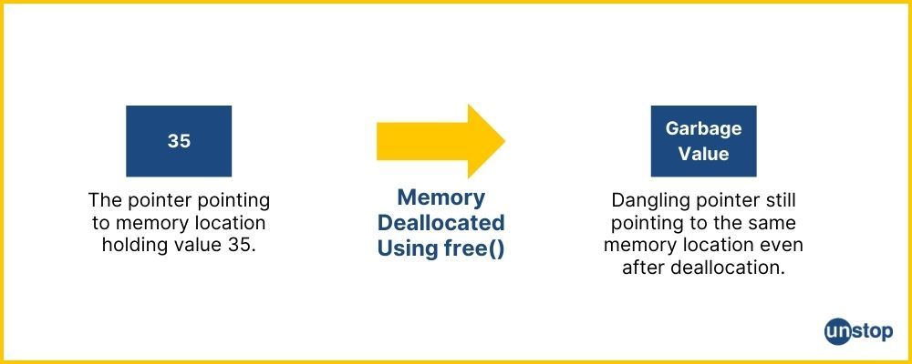
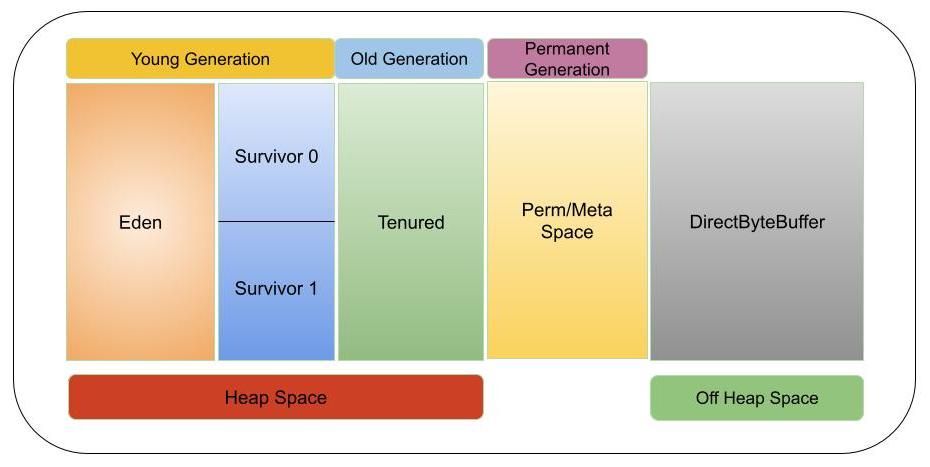
recommend-type

实现实时监控告警系统:Kafka与Grafana整合

![实现实时监控告警系统:Kafka与Grafana整合](https://imgconvert.csdnimg.cn/aHR0cHM6Ly9tbWJpei5xcGljLmNuL21tYml6X2pwZy9BVldpY3ladXVDbEZpY1pLWmw2bUVaWXFUcEdLT1VDdkxRSmQxZXB5R1lxaWNlUjA2c0hFek5Qc3FyRktudFF1VDMxQVl3QTRXV2lhSWFRMEFRc0I1cW1ZOGcvNjQw?x-oss-process=image/format,png) # 1.1 Kafka集群架构 Kafka集群由多个称为代理的服务器组成,这
recommend-type

解释这行代码 c = ((double)rand() / RAND_MAX) * (a + b - fabs(a - b)) + fabs(a - b);

这行代码的作用是随机生成一个浮点数,范围在 a 和 b 之间(包括 a 和 b)。 其中,`rand()` 函数是 C 语言标准库中的一个函数,用于生成一个伪随机整数。`RAND_MAX` 是一个常量,它表示 `rand()` 函数生成的随机数的最大值。 因此,`(double)rand() / RAND_MAX` 表示生成的随机数在 [0, 1] 之间的浮点数。 然后,将这个随机数乘上 `(a - b) - fabs(a - b)`,再加上 `fabs(a - b)`。 `fabs(a - b)` 是 C 语言标准库中的一个函数,用于计算一个数的绝对值。因此,`fabs(a - b)