A = np.array([[2.0, 1.0, 1.0], [4.0, -6.0, 0.0], [-2.0, 7.0, 2.0]]) b = np.array([5.0, -2.0, 9.0])
时间: 2023-07-02 14:13:57 浏览: 52
这个例子中,我们可以表示矩阵 $A$ 和向量 $b$,然后使用 NumPy 中的 `linalg.solve()` 函数来求解线性方程组 $Ax=b$。具体代码如下:
```python
import numpy as np
# 定义矩阵 A 和向量 b
A = np.array([[2.0, 1.0, 1.0],
[4.0, -6.0, 0.0],
[-2.0, 7.0, 2.0]])
b = np.array([5.0, -2.0, 9.0])
# 求解线性方程组 Ax=b
x = np.linalg.solve(A, b)
# 打印解向量 x
print("x =")
print(x)
```
输出:
```
x =
[ 2. -1. 3.]
```
其中,`np.linalg.solve()` 函数用于求解线性方程组。在这个例子中,我们定义了一个 $3\times 3$ 的矩阵 $A$ 和一个长度为 3 的向量 $b$,然后使用 `np.linalg.solve(A, b)` 求解线性方程组 $Ax=b$,并将结果存储在向量 $x$ 中。最后,我们打印出解向量 $x$。
相关问题
import numpy as np def dense(a_in, W, b, g): units = W.shape[0] a_out = np.zeros(units) for j in range(units): w = W[j] z = np.dot(w, a_in) + b[j] a_out[j] = g(z) return a_out def sequential(x): W1 = np.array([[1,-3,5], [2,4,-6]]) b1 = np.array([-1,1,2]) W2 = np.array([[-1,2], [3,-4], [-5,6]]) b2 = np.array([2,-2]) W3 = np.array([[-2,1], [3,-4]]) b3 = np.array([1,-2]) W4 = np.array([[3,-1]]) b4 = np.array([-2]) a1 = dense(x, W1, b1, np.tanh) a2 = dense(a1, W2, b2, np.tanh) a3 = dense(a2, W3, b3, np.tanh) a4 = dense(a3, W4, b4, np.tanh) f_x = a4 return f_x a_in = np.array([-2, 4]) print(sequential(a_in))
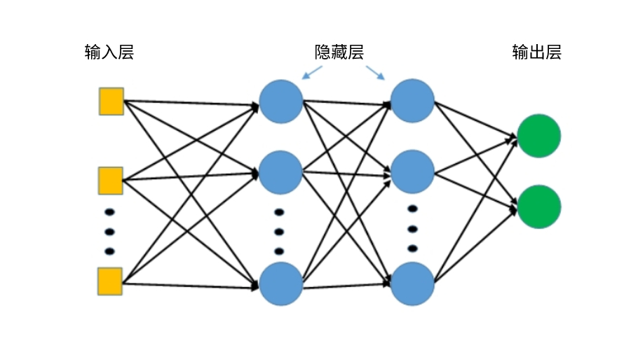
这段代码是一个神经网络的前向传播过程,包括了四个全连接层(dense)和四个激活函数(np.tanh),将输入向量a_in经过多次线性变换和非线性变换后,得到输出向量f_x。其中,每个全连接层的参数(权重W和偏置b)都是事先确定好的,依次为W1, b1, W2, b2, W3, b3, W4, b4。这个神经网络的输入维度为2,输出维度为1。通过执行这段代码,可以得到神经网络对输入a_in的预测输出。
import numpy as np array1 = np.array([1, 2, 3]) array2 = np.array([4, 5, 6]) x=np.sum(abs(array1-array2)>=-3) x的结果
根据提供的引用内容,可以得出以下答案:
```python
import numpy as np
array1 = np.array([1, 2, 3])
array2 = np.array([4, 5, 6])
x = np.sum(abs(array1 - array2) >= -3)
```
在上述代码中,`x`的结果是2。
相关推荐
最新推荐
基于网络的入侵检测系统源码+数据集+详细文档(高分毕业设计).zip
基于网络的入侵检测系统源码+数据集+详细文档(高分毕业设计).zip个人经导师指导并认可通过的高分毕业设计项目,评审分98分。主要针对计算机相关专业的正在做毕设的学生和需要项目实战练习的学习者,也可作为课程设计、期末大作业。
基于网络的入侵检测系统源码+数据集+详细文档(高分毕业设计).zip基于网络的入侵检测系统源码+数据集+详细文档(高分毕业设计).zip基于网络的入侵检测系统源码+数据集+详细文档(高分毕业设计).zip基于网络的入侵检测系统源码+数据集+详细文档(高分毕业设计).zip基于网络的入侵检测系统源码+数据集+详细文档(高分毕业设计).zip基于网络的入侵检测系统源码+数据集+详细文档(高分毕业设计).zip基于网络的入侵检测系统源码+数据集+详细文档(高分毕业设计).zip基于网络的入侵检测系统源码+数据集+详细文档(高分毕业设计).zip基于网络的入侵检测系统源码+数据集+详细文档(高分毕业设计).zip基于网络的入侵检测系统源码+数据集+详细文档(高分毕业设计).zip基于网络的入侵检测系统源码+数据集+详细文档(高分毕业设计).zip基于网络的入侵检测系统
本户型为2层独栋别墅D026-两层-13.14&12.84米-施工图.dwg
本户型为2层独栋别墅,建筑面积239平方米,占地面积155平米;一层建筑面积155平方米,设有客厅、餐厅、厨房、卧室3间、卫生间1间、杂物间;二层建筑面积84平方米,设有卧室2间、卫生间1间、储藏间、1个大露台。
本户型外观造型别致大方,采光通风良好,色彩明快,整体平面布局紧凑、功能分区合理,房间尺度设计适宜,豪华大气,富有时代气息。
Java_带有可选web的开源命令行RatioMaster.zip
Java_带有可选web的开源命令行RatioMaster
基于MATLAB实现的OFDM经典同步算法之一Park算法仿真,附带Park算法经典文献+代码文档+使用说明文档.rar
CSDN IT狂飙上传的代码均可运行,功能ok的情况下才上传的,直接替换数据即可使用,小白也能轻松上手
【资源说明】
基于MATLAB实现的OFDM经典同步算法之一Park算法仿真,附带Park算法经典文献+代码文档+使用说明文档.rar
1、代码压缩包内容
主函数:main.m;
调用函数:其他m文件;无需运行
运行结果效果图;
2、代码运行版本
Matlab 2020b;若运行有误,根据提示GPT修改;若不会,私信博主(问题描述要详细);
3、运行操作步骤
步骤一:将所有文件放到Matlab的当前文件夹中;
步骤二:双击打开main.m文件;
步骤三:点击运行,等程序运行完得到结果;
4、仿真咨询
如需其他服务,可后台私信博主;
4.1 期刊或参考文献复现
4.2 Matlab程序定制
4.3 科研合作
功率谱估计:
故障诊断分析:
雷达通信:雷达LFM、MIMO、成像、定位、干扰、检测、信号分析、脉冲压缩
滤波估计:SOC估计
目标定位:WSN定位、滤波跟踪、目标定位
生物电信号:肌电信号EMG、脑电信号EEG、心电信号ECG
通信系统:DOA估计、编码译码、变分模态分解、管道泄漏、滤波器、数字信号处理+传输+分析+去噪、数字信号调制、误码率、信号估计、DTMF、信号检测识别融合、LEACH协议、信号检测、水声通信
5、欢迎下载,沟通交流,互相学习,共同进步!
基于MATLAB实现的对机械振动信号用三维能量谱进行分析+使用说明文档.rar
CSDN IT狂飙上传的代码均可运行,功能ok的情况下才上传的,直接替换数据即可使用,小白也能轻松上手
【资源说明】
基于MATLAB实现的对机械振动信号用三维能量谱进行分析+使用说明文档.rar
1、代码压缩包内容
主函数:main.m;
调用函数:其他m文件;无需运行
运行结果效果图;
2、代码运行版本
Matlab 2020b;若运行有误,根据提示GPT修改;若不会,私信博主(问题描述要详细);
3、运行操作步骤
步骤一:将所有文件放到Matlab的当前文件夹中;
步骤二:双击打开main.m文件;
步骤三:点击运行,等程序运行完得到结果;
4、仿真咨询
如需其他服务,可后台私信博主;
4.1 期刊或参考文献复现
4.2 Matlab程序定制
4.3 科研合作
功率谱估计:
故障诊断分析:
雷达通信:雷达LFM、MIMO、成像、定位、干扰、检测、信号分析、脉冲压缩
滤波估计:SOC估计
目标定位:WSN定位、滤波跟踪、目标定位
生物电信号:肌电信号EMG、脑电信号EEG、心电信号ECG
通信系统:DOA估计、编码译码、变分模态分解、管道泄漏、滤波器、数字信号处理+传输+分析+去噪、数字信号调制、误码率、信号估计、DTMF、信号检测识别融合、LEACH协议、信号检测、水声通信
5、欢迎下载,沟通交流,互相学习,共同进步!
zigbee-cluster-library-specification
最新的zigbee-cluster-library-specification说明文档。
管理建模和仿真的文件
管理Boualem Benatallah引用此版本:布阿利姆·贝纳塔拉。管理建模和仿真。约瑟夫-傅立叶大学-格勒诺布尔第一大学,1996年。法语。NNT:电话:00345357HAL ID:电话:00345357https://theses.hal.science/tel-003453572008年12月9日提交HAL是一个多学科的开放存取档案馆,用于存放和传播科学研究论文,无论它们是否被公开。论文可以来自法国或国外的教学和研究机构,也可以来自公共或私人研究中心。L’archive ouverte pluridisciplinaire
【实战演练】MATLAB用遗传算法改进粒子群GA-PSO算法
# 2.1 遗传算法的原理和实现
遗传算法(GA)是一种受生物进化过程启发的优化算法。它通过模拟自然选择和遗传机制来搜索最优解。
**2.1.1 遗传算法的编码和解码**
编码是将问题空间中的解表示为二进制字符串或其他数据结构的过程。解码是将编码的解转换为问题空间中的实际解的过程。常见的编码方法包括二进制编码、实数编码和树形编码。
**2.1.2 遗传算法的交叉和
openstack的20种接口有哪些
以下是OpenStack的20种API接口:
1. Identity (Keystone) API
2. Compute (Nova) API
3. Networking (Neutron) API
4. Block Storage (Cinder) API
5. Object Storage (Swift) API
6. Image (Glance) API
7. Telemetry (Ceilometer) API
8. Orchestration (Heat) API
9. Database (Trove) API
10. Bare Metal (Ironic) API
11. DNS
JSBSim Reference Manual
JSBSim参考手册,其中包含JSBSim简介,JSBSim配置文件xml的编写语法,编程手册以及一些应用实例等。其中有部分内容还没有写完,估计有生之年很难看到完整版了,但是内容还是很有参考价值的。