没有合适的资源?快使用搜索试试~ 我知道了~
首页气候研究统计分析入门与应用指南
气候研究统计分析入门与应用指南
需积分: 9 6 下载量 114 浏览量
更新于2024-07-17
收藏 11.59MB PDF 举报
"《统计分析在气候研究中的应用》是由汉斯·冯·施托尔希(Hans von Storch)和弗朗西斯·W·齐尔斯(Francis W. Zwiers)合著的一本专业书籍,由剑桥大学出版社出版。该书的核心目标是为气候学家提供深入理解统计学原理的途径,帮助他们正确、有效地运用统计方法进行气候科学研究。书中内容全面,包括基础介绍、标准高级技术以及专为气候学家设计的特殊技术,所有这些都在一个单一的资源中得到了整合。 气候学本质上是对我们气候的统计学研究,因此数学统计学的威力在气候研究中广泛应用,涵盖了从简单地确定气候学平均值的不确定性到揭示气候系统动态的复杂技术。作者通过大量来自气候科学文献的实际案例,生动展示了统计分析在气候研究中的必要性、力量以及可能遇到的陷阱。这本书不仅适合作为研究生课程的主要教材,针对气候学、大气科学和海洋科学的学生,也适合那些希望提升统计技能的气候研究人员。 书中深入浅出地讲解了基本的统计原则,如假设检验、回归分析、时间序列分析等,并强调了在实际研究中如何选择和解释统计结果的重要性。此外,它还探讨了如何处理气候变化数据的异质性、非线性关系以及潜在的多重共线性问题,这些都是气候科学家在应用统计时必须面对的挑战。 通过阅读本书,气候研究人员可以提高其数据分析的精度和可靠性,同时增强对不确定性和模型偏差的理解。《统计分析在气候研究中的应用》是一本既实用又具有理论深度的参考书,对于推动气候科学研究的进步具有重要意义。"
资源详情
资源推荐
1.2: Some Typical Problems and Concepts
5
Figure 1.2: The monthly mean Southern Oscillation Index, computed as the difference between Darwin
(Australia) and Papeete (Tahiti) monthly mean sea-level pressure (‘Jahr’ is German for ‘year’).
Figure 1.3: Auto-correlation function of the index shown in Figure 1.2. Units: %.
channels might be:
e
1t
= α
1
(t − t
0
) + ²
1t
,
e
2t
= α
2
(t − t
0
) + ²
2t
,
where t
0
is the launch time of the satellite and
α
1
and α
2
are fixed constants describing the rates
of drift of the two radiometers. The instrumental
errors, ²
1t
and ²
2t
, are statistically independent of
each other, implying that the correlation between
the two, ρ(²
1t
,²
2t
), is zero. Consequently the
total errors, e
1t
and e
2t
, are also statistically
independent even though they share a common
systematic component. However, simple estimates
of correlation between e
1t
and e
2t
that do not
account for the deterministic drift will suggest that
these two quantities are correlated.
Correlations manifest themselves in several dif-
ferent ways in observed and simulated climates.
Several adjectives are used to describe corre-
lations depending upon whether they describe
relationships in time (serial correlation, lagged
correlation), space (spatial correlation, telecon-
nection), or between different climate variables
(cross-correlation).
A good example of serial correlation is the
monthly Southern Oscillation Index (SOI),
6
which
6
The Southern Oscillation is the major mode of natural
climate variability on the interannual time scale. It is frequently
used as an example in this book.
It has been known since the end of the last century
(Hildebrandson [177]; Walker, 1909–21) that sea-level pressure
(SLP) in the Indonesian region is negatively correlated with that
over the southeast tropical Pacific. A positive SLP anomaly
6
1: Introduction
is defined as the anomalous monthly mean
pressure difference between Darwin (Australia)
and Papeete (Tahiti) (Figure 1.2).
The time series is basically stationary, although
variability during the first 30 years seems to be
somewhat weaker than that of late. Despite the
noisy nature of the time series, there is a distinct
tendency for the SOI to remain positive or negative
for extended periods, some of which are indicated
in Figure 1.2. This persistence in the sign of the
index reflects the serial correlation of the SOI.
A quantitative measure of the serial correlation
is the auto-correlation function, ρ
SOI
(t, t + 1),
shown in Figure 1.3, which measures the similarity
of the SOI at any time difference 1. The auto-
correlation is greater than 0.2 for lags up to
about six months and varies smoothly around zero
with typical magnitudes between 0.05 and 0.1
for lags greater than about a year. This tendency
of estimated auto-correlation functions not to
converge to zero at large lags, even though the
real auto-correlation is zero at long lags, is a
natural consequence of the uncertainty due to finite
samples (see Section 11.1).
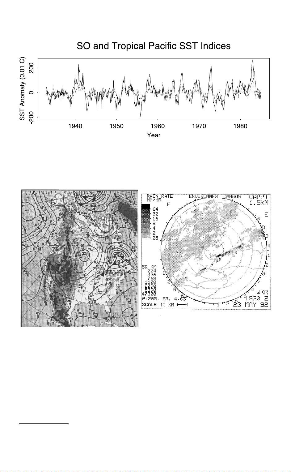
A good example of a cross-correlation is the
relationship that exists between the SOI and
various alternative indices of the Southern Os-
cillation [426]. The characteristic low-frequency
variations in Figure 1.2 are also present in area-
averaged Central Pacific sea-surface temperature
(Figure 1.4).
7
The correlation between the two
time series displayed in Figure 1.4 is 0.67.
Pattern analysis techniques, such as Empiri-
cal Orthogonal Function analysis (Chapter 13),
Canonical Correlation Analysis (Chapter 14) and
Principal Oscillation Patterns (Chapter 15), rely
upon the assumption that the fields under study are
(i.e., a deviation from the long-term mean) over, say, Darwin
(Northern Australia) tends to be associated with a negative
SLP anomaly over Papeete (Tahiti). This seesaw is called
the Southern Oscillation (SO). The SO is associated with
large-scale and persistent anomalies of sea-surface temperature
in the central and eastern tropical Pacific (El Ni
˜
no and
La Ni
˜
na). Hence the phenomenon is often referred to as
the ‘El Ni
˜
no/Southern Oscillation’ (ENSO). Large zonal
displacements of the centres of precipitation are also associated
with ENSO. They reflect anomalies in the location and intensity
of the meridionally (i.e., north–south) oriented Hadley cell and
of the zonally oriented Walker cell.
The state of the Southern Oscillation may be monitored with the
monthly SLP difference between observations taken at surface
stations in Darwin, Australia and Papeete, Tahiti. It has become
common practice to call this difference the Southern Oscillation
Index (SOI) although there are also many other ways to define
equivalent indices [426].
7
Other definitions, such as West Pacific rainfall, sea-level
pressure at Darwin alone or the surface zonal wind in the central
Pacific, also yield indices that are highly correlated with the
usual SOI. See Wright [427].
spatially correlated. The Southern Oscillation In-
dex (Figure 1.2) is a manifestation of the negative
correlation between surface pressure at Papeete
and that at Darwin. Variables such as pressure,
height, wind, temperature, and specific humidity
vary smoothly in the free atmosphere and con-
sequently exhibit strong spatial interdependence.
This correlation is present in each weather map
(Figure 1.5, left). Indeed, without this feature,
routine weather forecasts would be all but impos-
sible given the sparseness of the global observing
network as it exists even today. Variables derived
from moisture, such as cloud cover, rainfall and
snow amounts, and variables associated with land
surface processes tend to have much smaller spa-
tial scales (Figure 1.5, right), and also tend not to
have normal distributions (Sections 3.1 and 3.2).
While mean sea-level pressure (Figure 1.5, left)
will be more or less constant on spatial scales of
tens of kilometres, we may often travel in and out
of localized rain showers in just a few kilometres.
This dichotomy is illustrated in Figure 1.5, where
we see a cold front over Ontario (Canada). The
left panel, which displays mean sea-level pressure,
shows the front as a smooth curve. The right panel
displays a radar image of precipitation occurring
in southern Ontario as the front passes through the
region.
1.2.3 Stationarity, Cyclo-stationarity, and Non-
stationarity. An important concept in statistical
analysis is stationarity. A random variable, or a
random process, is said to be stationary if all
of its statistical parameters are independent of
time. Most statistical techniques assume that the
observed process is stationary.
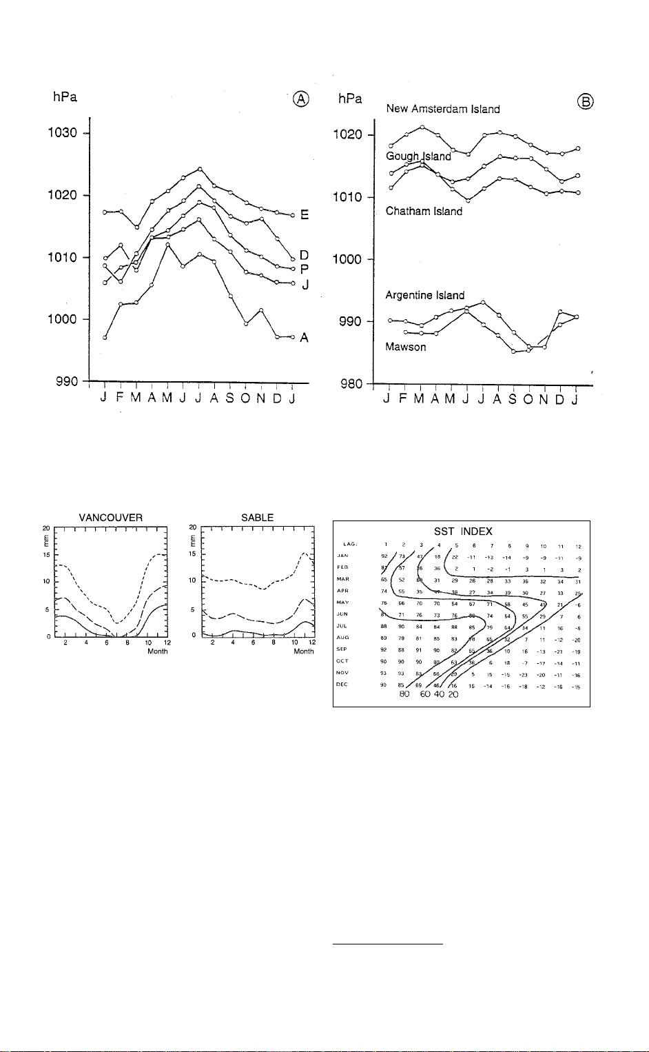
However, most climate parameters that are
sampled more frequently than one per year are
not stationary but cyclo-stationary, simply because
of the seasonal forcing of the climate system.
Long-term averages of monthly mean sea-level
pressure exhibit a marked annual cycle, which is
almost sinusoidal (with one maximum and one
minimum) in most locations. However, there are
locations (Figure 1.6) where the annual cycle is
dominated by a semiannual variation (with two
maxima and minima). In most applications the
mean annual cycle is simply subtracted from the
data before the remaining anomalies are analysed.
The process is cyclo-stationary in the mean if it is
stationary after the annual cycle has been removed.
Other statistical parameters (e.g., the percentiles
of rainfall) may also exhibit cyclo-stationary
behaviour. Figure 1.7 shows the annual cycles
1.2: Some Typical Problems and Concepts
7
Figure 1.4: The conventional Southern Oscillation Index (SOI = pressure difference between Darwin
and Tahiti; dashed curve) and a sea-surface temperature (SST) index of the Southern Oscillation (solid
curve) plotted as a function of time. The conventional SOI has been doubled in this figure.
Figure 1.5: State of the atmosphere over North America on 23 May 1992.
Left: Analysis of the sea-level pressure field (12:00 UTC (Universal Time Coordinated); from
Europ
¨
aisher Wetterbericht 17, Band 144; with permission of the Deutsher Wetterdienst).
Right: Weather radar image, showing rainfall rates, for southern Ontario (19:30 local time; courtesy
Paul Joe, AES Canada [94].)
Note that the radar image and the weather map refer to different times, namely 12:00 UTC on 23 May
and 00:30 UTC on 24 May.
of the 70th, 80th, and 90th percentiles
8
of 24-
hour rainfall amounts for each calendar month at
8
Or ‘quantiles,’ that is, thresholds selected so that 70%,
80%, or 90% of all 24-hour rainfall amounts are less than the
respective threshold [2.6.4].
Vancouver (British Columbia) and Sable Island
(off the coast of Nova Scotia) [450].
The Southern Oscillation Index is not strictly
stationary. Wright [427] showed that the linear
serial correlation of the SOI depends upon the time
8
1: Introduction
Figure 1.6: Annual cycle of sea-level pressure at extratropical locations.
a) Northern Hemisphere Ocean Weather Stations: A = 62
◦
N, 33
◦
W;D=44
◦
N, 41
◦
W; E = 35
◦
N,
48
◦
W;J=52
◦
N, 25
◦
W;P=50
◦
N, 145
◦
W.
b) Southern Hemisphere.
Figure 1.7: Monthly 90th, 80th, and 70th per-
centiles (from top to bottom) of 24-hour rainfall
amounts at Vancouver and Sable Island [450].
of the year. The serial correlation is plotted as a
function of time of year and lag in Figure 1.8.
Correlations between values of the SOI in May
and values in subsequent months decay slowly
with increasing lag, while similar correlations with
values in April decay quickly. Because of this
behaviour, Wright defined an ENSO year that
begins in May and ends in April.
Regular observations taken over extended
periods at a certain station sometimes exhibit
changes in their statistical properties. These might
be abrupt or gradual (such as changes that might
occur when the exposure of a rain gauge changes
slowly over time, as a consequence of the growth
of vegetation or changes in local land use). Abrupt
Figure 1.8: Seasonal dependence of the lag
correlations of the SST index of the Southern
Oscillation. The correlations are given in hundreds
so that isolines represent lag correlations of 0.8,
0.6, 0.4, and 0.2. The row labelled ‘Jan’ lists
correlations between January values of the index
and the index observed later ‘lag’ months [427].
changes in the observational record may take
place if the instrument (or the observer) changes,
the site is moved,
9
or recording practices are
changed. Such non-natural or artificial changes are
9
Karl et al. [213] describe a case in which a precipitation
gauge recorded significantly different values after being raised
one metre from its original position.
1.2: Some Typical Problems and Concepts
9
Figure 1.9: Annual mean daily minimum temper-
ature time series at two neighbouring sites in
Quebec. Sherbrooke has experienced considerable
urbanization since the beginning of the century
whereas Shawinigan has maintained more of its
rural character.
Top: The raw records. The abrupt drop of several
degrees in the Sherbrooke series in 1963 reflects
the move of the instrument from downtown Sher-
brooke to its suburban airport. The reason for
the downward dip before 1915 in the Shawinigan
record is unknown.
Bottom: Corrected time series for Sherbrooke
and Shawinigan. The Sherbrooke data from 1963
onward are increased by 3.2
◦
C. The straight lines
are trend lines fitted to the corrected Sherbrooke
data and the 1915–90 Shawinigan record.
Courtesy L. Vincent, AES Canada.
called inhomogeneities. An example is contained
in the temperature records of Sherbrooke and
Shawinigan (Quebec) shown in the upper panel
of Figure 1.9. The Sherbrooke observing site
was moved from a downtown location to a
suburban airport in 1963—and the recorded
temperature abruptly dropped by more than 3
◦
C.
The Shawinigan record may also be contaminated
by observational errors made before 1915.
Geophysical time series often exhibit a trend.
Such trends can originate from various sources.
One source is urbanization, that is, the increasing
density and height of buildings around an obser-
vation location and the corresponding changes in
the properties of the land surface. The temper-
ature at Sherbrooke, a location heavily affected
by development, exhibits a marked upward trend
after correction for the systematic change in 1963
(Figure 1.9, bottom). This temperature trend is
much weaker for the neighbouring Shawinigan,
perhaps due to a weaker urbanization effect at that
site or natural variations of the climate system.
Both temperature trends at Sherbrooke and Shaw-
inigan are real, not observational artifacts. The
strong trend at Sherbrooke must not be mistaken
for an indication of global warming.
Trends in the large-scale state of the climate
system may reflect systematic forcing changes
of the climate system (such as variations in the
Earth’s orbit, or increased CO
2
concentration
in the atmosphere) or low-frequency internally
generated variability of the climate system. The
latter may be deceptive because low-frequency
variability, on short time series, may be mistakenly
interpreted as trends. However, if the length of
such time series is increased, a metamorphosis
of the former ‘trend’ takes place and it becomes
apparent that the trend is a part of the natural
variation of the system.
10
1.2.4 Quality of Forecasts. The Old Farmer’s
Almanac publishes regular outlooks for the climate
for the coming year. The method used to prepare
these outlooks is kept secret, and scientists
question the existence of skill in the predictions.
To determine whether these skeptics are right or
wrong, measures of the skill of the forecasting
scheme are needed. These skill scores can be used
to compare forecasting schemes objectively.
The Almanac makes categorical forecasts of
future temperature and precipitation amount in
two categories, ‘above’ or ‘below’ normal. A
suitable skill score in this case is the number of
correct forecasts. Trivial forecasting schemes such
as persistence (no change), climatology, or pure
chance can be used as reference forecasts if no
other forecasting scheme is available. Once we
have counted the number of correct forecasts made
with both the tested and the reference schemes, we
can estimate the improvement (or degradation) of
forecast skill by computing the difference in the
counts. Relatively simple probabilistic methods
can be used to make a judgement about the
10
This is an example of the importance of time scales
in climate research, an illustration that our interpretation of
a given process depends on the time scales considered. A
short-term trend may be just another swing in a slowly varying
system. An example is the Madden-and-Julian Oscillation
(MJO, [264]), which is the strongest intra-seasonal mode in the
tropical troposphere. It consists of a wavenumber 1 pattern that
travels eastward round the globe. The MJO has a mean period
of 45 days and has significant memory on time scales of weeks;
on time scales of months and years, however, the MJO has no
temporal correlation.
剩余494页未读,继续阅读
DISCIPVLVS
- 粉丝: 0
- 资源: 3
上传资源 快速赚钱
- 我的内容管理 展开
- 我的资源 快来上传第一个资源
- 我的收益 登录查看自己的收益
- 我的积分 登录查看自己的积分
- 我的C币 登录后查看C币余额
- 我的收藏
- 我的下载
- 下载帮助
最新资源
- Hadoop生态系统与MapReduce详解
- MDS系列三相整流桥模块技术规格与特性
- MFC编程:指针与句柄获取全面解析
- LM06:多模4G高速数据模块,支持GSM至TD-LTE
- 使用Gradle与Nexus构建私有仓库
- JAVA编程规范指南:命名规则与文件样式
- EMC VNX5500 存储系统日常维护指南
- 大数据驱动的互联网用户体验深度管理策略
- 改进型Booth算法:32位浮点阵列乘法器的高速设计与算法比较
- H3CNE网络认证重点知识整理
- Linux环境下MongoDB的详细安装教程
- 压缩文法的等价变换与多余规则删除
- BRMS入门指南:JBOSS安装与基础操作详解
- Win7环境下Android开发环境配置全攻略
- SHT10 C语言程序与LCD1602显示实例及精度校准
- 反垃圾邮件技术:现状与前景
资源上传下载、课程学习等过程中有任何疑问或建议,欢迎提出宝贵意见哦~我们会及时处理!
点击此处反馈
安全验证
文档复制为VIP权益,开通VIP直接复制
信息提交成功