

Explainable Deep Learning Methods in Medical Diagnosis: A Survey • 7
understand the contribution of dierent features in the model prediction, or by analytically determining the
contribution of dierent features to the model prediction. On the other hand, intrinsic models, also known as
in-model approaches or inherently interpretable models are self-explainable since they are designed to produce
human-understandable representations from the internal model features.
3.2 Classical XAI Methods
The rst attempts to explain deep learning models relied on the post-hoc analysis of the models. In spite of the
criticism that post-hoc approaches have been recently subjected [
105
], they are still being used in many domains
of medical imaging, and their understanding is important to explain the advances on the topic of interpretable
deep learning. As such, the following sections briey describe the most popular XAI algorithms according to the
two major categories of post-hoc analysis.
3.2.1 Perturbation-based methods. The rationale behind perturbation-based methods is to perceive how a
perturbation in the input aects the model’s prediction. Two of the most representative perturbation-based
methods are LIME [101] and SHAP [77]; and an occlusion-based method [151].
LIME
. LIME [
101
] stands for Local Interpretable Model-agnostic Explanations. As the name suggests, it can
explain any black-box model, and according to the XAI taxonomy is a post-hoc, model-agnostic method providing
local explanations. The intuition behind LIME is to approximate the complex model (black-box model) locally
with an interpretable model, usually denoted as local surrogate model. Thus, an individual instance is explained
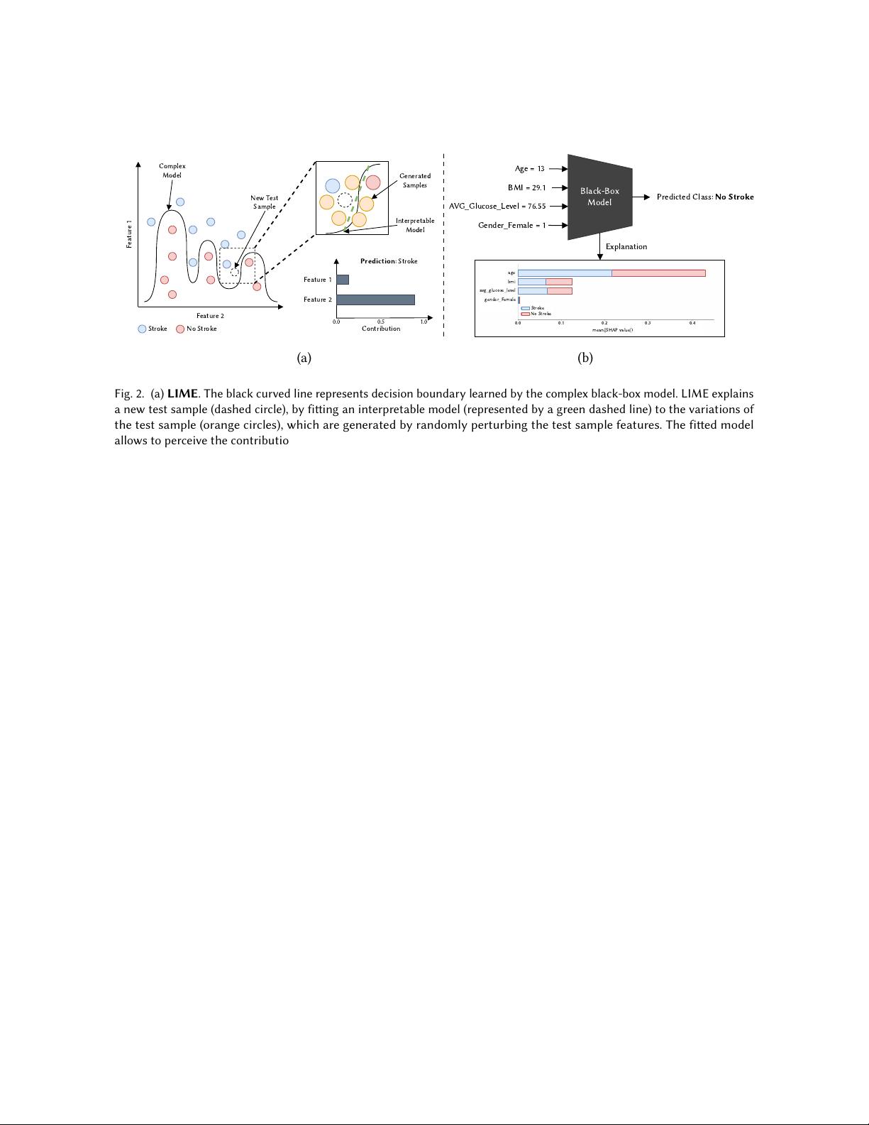
locally using a simple interpretable model around the prediction, such as linear models or decision trees. Figure 2
a) provides an intuitive illustration of the overall functioning of LIME.
In order to approximate the model prediction locally, a new dataset consisting of perturbed samples conditioned
on their proximity to the instance being explained is used to t the interpretable model. The labels for those
perturbed samples are obtained through the complex model. In the case of tabular data, the perturbed instances
are sampled around the instance being explained, by randomly changing the feature values in order to obtain
samples both in the vicinity and far away from the instance being explained. Analogously, when LIME is applied
to the image classication problem, the image being explained is rst segmented into superpixels, which are
groups of pixels in the image sharing common characteristics, such as colour and intensity. Then, the perturbed
versions of the original data are obtained by randomly masking out a subset of superpixels, resulting in an
image with occluded patches. The new dataset used to t the interpretable model consists of perturbed versions
of the image being explained, and the superpixels with the highest positive coecients in the interpretable
model suggest they largely contributed to the prediction. Thus, they will be selected as part of the interpretable
representation that is simple a binary vector indicating the presence or absence of those superpixels.
SHAP
. SHAP [
77
] was inspired on the Shapley values from the cooperative game theory [
113
] and operates
by determining the average contribution of a feature value to the model prediction using all combinations of the
features powerset. As an example, given the task of predicting the risk of stroke based on age, gender and Body
Mass Index (BMI), the SHAP explanations for a particular prediction are given in terms of the contribution of
each feature. This contribution is determined from the change observed in model prediction when using the 2
𝑛
combinations from the features powerset, where the missing features are replaced by random values. Figure 2 b)
illustrates the above-described example. Similar to LIME, SHAP is a local model-agnostic interpretation method
that can be applied to both tabular and image data. In the case of tabular data, the explanation is given in the
form of importance values to each feature. In the case of image data, it follows a similar procedure to the LIME,
by calculating the Shapley values for all possible combinations between superpixels. Several variations of SHAP
method were proposed to approximate Shapley values in a more ecient way, namely KernelSHAP, DeepSHAP
and TreeSHAP [76].
, Vol. 1, No. 1, Article . Publication date: May 2022.
剩余35页未读,继续阅读

努力+努力=幸运
- 粉丝: 2
- 资源: 138
 我的内容管理
收起
我的内容管理
收起
- 我的资源
快来上传第一个资源
 我的收益 登录查看自己的收益
 我的积分
登录查看自己的积分
我的积分
登录查看自己的积分
 我的C币
登录后查看C币余额
我的C币
登录后查看C币余额
 我的收藏
我的收藏  我的下载
我的下载  下载帮助
下载帮助

会员权益专享


最新资源
- 京瓷TASKalfa系列维修手册:安全与操作指南
- 小波变换在视频压缩中的应用
- Microsoft OfficeXP详解:WordXP、ExcelXP和PowerPointXP
- 雀巢在线媒介投放策划:门户网站与广告效果分析
- 用友NC-V56供应链功能升级详解(84页)
- 计算机病毒与防御策略探索
- 企业网NAT技术实践:2022年部署互联网出口策略
- 软件测试面试必备:概念、原则与常见问题解析
- 2022年Windows IIS服务器内外网配置详解与Serv-U FTP服务器安装
- 中国联通:企业级ICT转型与创新实践
- C#图形图像编程深入解析:GDI+与多媒体应用
- Xilinx AXI Interconnect v2.1用户指南
- DIY编程电缆全攻略:接口类型与自制指南
- 电脑维护与硬盘数据恢复指南
- 计算机网络技术专业剖析:人才培养与改革
- 量化多因子指数增强策略:微观视角的实证分析
资源上传下载、课程学习等过程中有任何疑问或建议,欢迎提出宝贵意见哦~我们会及时处理!
点击此处反馈


