机械系统高级滑模控制设计与MATLAB仿真
需积分: 26 127 浏览量
更新于2024-07-17
1
收藏 4.17MB PDF 举报
"Advanced Sliding Mode Control for Mechanical Systems: A Comprehensive Guide with MATLAB Simulations" 由Jinkun Liu 和 Xinhua Wang 联合编著,这本书是一本深入研究高级滑模控制在机械系统设计、分析以及MATLAB仿真中的应用的专业著作。全书共分为12个章节,涵盖了滑模变结构控制的基础设计理念,如基于标称模型的滑模控制,利用线性矩阵不等式和反演滑模技术的控制策略,还有离散、动态、自适应、终端、基于观测器的滑模控制方法。此外,书中特别关注了模糊滑模控制和神经网络滑模控制在实际机械系统中的应用,例如在飞机和机器人领域的实例。
每一章节都详尽地探讨了理论原理,并辅以165幅清晰的图表,帮助读者更好地理解和掌握各种控制方法。两位作者分别来自北京航空航天大学和新加坡国立大学,他们的学术背景为本书提供了深厚的专业基础。该书由中国清华大学出版社和Springer-Verlag Berlin Heidelberg联合出版,强调版权保护,所有内容未经许可不得复制或再利用。
此书ISBN分别为978-7-302-24827-9(中文版)和978-3-642-20906-2(英文版),旨在提供给广大机械工程、自动化控制以及信号处理领域的专业人士一个全面且实践性强的学习工具。通过MATLAB的仿真案例,读者可以亲身体验如何将理论知识转化为实际控制系统的优化解决方案。对于那些寻求提升机械系统性能、探索新型控制策略的研究者和工程师来说,这是一本不可多得的参考书籍。

Advanced Sliding Mode Control for Mechanical Systems: Design, Analysis and MATLAB Simulation
2
(VSC) with sliding mode control. During the past decades, VSC and SMC have
generated significant interest in the control research community.
SMC has been applied into general design method being examined for wide
spectrum of system types including nonlinear system, multi-input multi-output
(MIMO) systems, discrete-time models, large-scale and infinite-dimension systems,
and stochastic systems. The most eminent feature of SMC is it is completely
insensitive to parametric uncertainty and external disturbances during sliding
mode
[2]
.
VSC utilizes a high-speed switching control law to achieve two objectives.
Firstly, it drives the nonlinear plant’s state trajectory onto a specified and user-
chosen surface in the state space which is called the sliding or switching surface.
This surface is called the switching surface because a control path has one gain if
the state trajectory of the plant is “above” the surface and a different gain if the
trajectory drops “below” the surface. Secondly, it maintains the plant’s state
trajectory on this surface for all subsequent times. During the process, the control
system’s structure varies from one to another and thereby earning the name
variable structure control. The control is also called as the sliding mode control
[3]
to emphasize the importance of the sliding mode.
Under sliding mode control, the system is designed to drive and then constrain
the system state to lie within a neighborhood of the switching function. Its two
main advantages are (1) the dynamic behavior of the system may be tailored by
the particular choice of switching function, and (2) the closed-loop response
becomes totally insensitive to a particular class of uncertainty. Also, the ability to
specify performance directly makes sliding mode control attractive from the
design perspective.
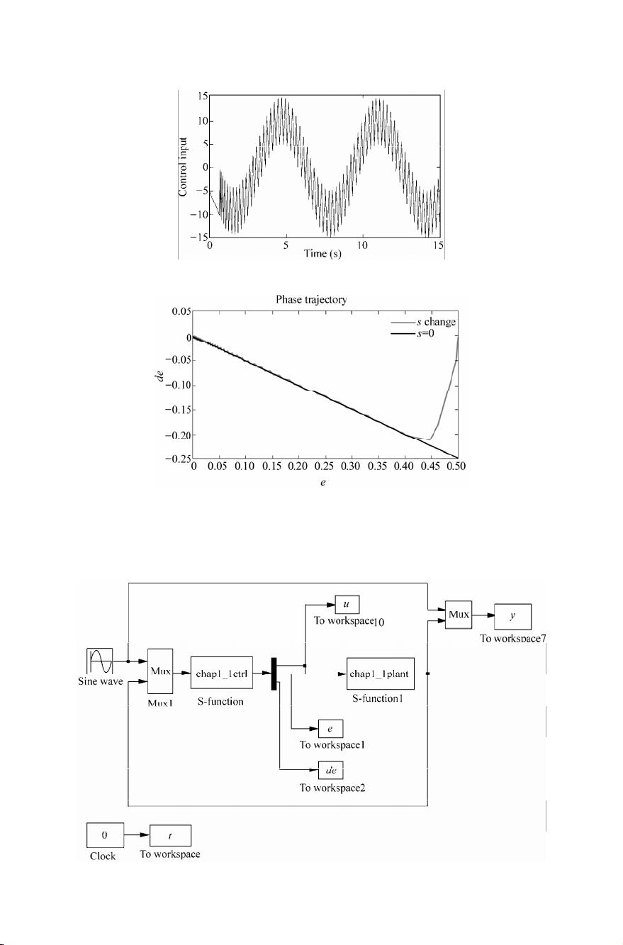
Trajectory of a system can be stabilized by a sliding mode controller. The
system states “slides” along the line
0s after the initial reaching phase. The
particular 0s surface is chosen because it has desirable reduced-order dynamics
when constrained to it. In this case, the
11
,
s
cx x
0c !
surface corresponds to
the first-order LTI system
11
,
x
cx
which has an exponentially stable origin. Now,
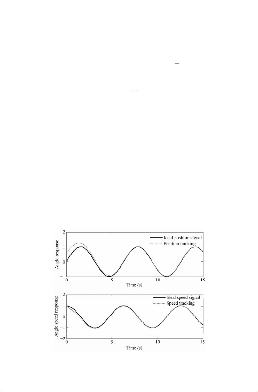
we consider a simple example of the sliding mode controller design as under.
Consider a plant as
() ()Jt ut
T
(1.1)
where
J
is the inertia moment, ()t
T
is the angle signal, and ( )ut is the control
input.
Firstly, we design the sliding mode function as
() () ()
s
tcetet
(1.2)
where
c
must satisfy the Hurwitz condition,
0.c !
The tracking error and its derivative value are
d
() () (),et t t
TT
d
() () ()et t t
TT


剩余365页未读,继续阅读
164 浏览量
178 浏览量
112 浏览量
116 浏览量
2018-09-21 上传
点击了解资源详情
点击了解资源详情
点击了解资源详情
点击了解资源详情

悠然
- 粉丝: 2
- 资源: 15
 我的内容管理
展开
我的内容管理
展开


最新资源
- GEN32“创世纪32“监控组态软件.rar
- valle-input:很棒的valle输入元素-使用Polymer 3x的Web组件
- Simple Picture Puzzle Game in JavaScript Free Source Code.zip
- ssm高考志愿填报系统设计毕业设计程序
- MyApplication:组件化、
- wc-core:Mofon Design的Web组件核心
- odrViewer.zip_odrViewer_opendrive_opendrive viewer_opendrive可视化_
- Simple Table Tennis Game using JavaScript
- 同步安装文件2.rar
- GalaxyFighters-开源
- STM32+W5500 Modbus-TCP协议功能实现
- Excel做为数据库登录的三层实现_dotnet整站程序.rar
- konsave:Konsave允许使用保存您的KDE Plasma自定义设置并非常轻松地还原它们!
- make-element:创建没有样板的自定义元素
- MachineLearning
- Simple Platformer Game using JavaScript
