非高斯噪声模型下的核岭回归及其应用
112 浏览量
更新于2024-08-29
收藏 1.02MB PDF 举报
"Kernel ridge regression for general noise model with its application"
这篇研究论文主要探讨了核岭回归在处理非高斯噪声模型中的应用。核岭回归(Kernel Ridge Regression, KRR)是一种常用的统计学习方法,它结合了岭回归和核方法的优点,能够处理非线性关系的数据。传统的岭回归假设噪声是高斯分布的,但在实际应用中,如短期风速预测等领域,噪声可能并不符合高斯分布。因此,这种假设在某些情况下可能导致预测性能的下降。
论文指出,当噪声模型不符合高斯分布时,经典的回归技术不再是最优选择。为了应对这个问题,作者提出了将核岭回归应用于更广泛的噪声模型,旨在提高预测的准确性和鲁棒性。这涉及到对损失函数的调整,以便更好地适应不同类型的噪声分布。损失函数是衡量预测误差的重要指标,它的设计直接影响到模型的性能。
文章还讨论了如何在核岭回归中引入等式约束(equality constraints),这可以进一步优化模型的训练过程。等式约束允许在满足特定条件的情况下进行回归分析,比如在某些变量之间存在固定的关系或限制。通过这种方式,模型可以更好地捕捉数据的内在结构。
在短期风速预测的例子中,作者可能展示了如何利用改进后的核岭回归来处理非高斯噪声,以提高预测精度。短期风速预测对于能源管理、航空安全等领域具有重要意义,因此,开发能够有效处理噪声的预测模型至关重要。
此外,论文可能还涉及了模型的训练策略、参数选择以及模型验证等方面,这些都是保证模型性能的关键环节。通过理论分析和实验结果,作者证明了他们的方法在处理非高斯噪声问题上的优势,并提供了实际应用的案例来支持这一观点。
这篇论文不仅对核岭回归的理论进行了扩展,使其能适应更广泛的实际噪声模型,还提供了实用的解决方案,有助于在实际问题中提升预测模型的性能。这对于机器学习和统计学领域的研究者以及依赖于预测分析的行业从业者都具有很高的参考价值。
In the Bayesian approach, we regard the function f as the
realization of a random field with a known prior probability
distribution. We are interested in maximizing the a posteriori
probability of f given the data D
f
, namely P½f jD
f
, which can be
written as
P½f jD
f
p P½D
f
jf P½f ; ð5Þ
where P½D
f
jf is the conditional probability of the data D
f
given the
function f and P½f is a priori probability of random field f, which is
often written as P½f p expð
λ Φ½f Þ, where Φ½ f is a smoothness
functional. The probability P½D
f
jf is essentially a model of the
noise, and if the noise is additive, as in Eq. (3) and i.i.d. with
probability distribution Pðe
i
Þ, P½D
f
jf can be written as
P½D
f
jf ¼ ∏
l
i ¼ 1
Pðe
i
Þ: ð6Þ
Substituting P½f and Eq. (6) in (5), maximizing the posterior
probability of f given the data D
f
is equal to minimizing the
following functional
H½f ¼ ∑
l
i ¼ 1
log ½Pðy
i
f ðx
i
ÞÞ e
λ
Φ
½f
¼ ∑
l
i ¼ 1
log Pðy
i
f ðx
i
ÞÞþλ Φ½f : ð7Þ
This functional is of the same form as Eq. (4) [29]. By Eqs.
(4) and (7), the optimal loss function in maximum a posteriori is
cðeÞ¼cðx; y; f ðxÞÞ ¼ log pðy f ðxÞÞ : ð8Þ
We assume that the noise in Eq. (3) is Laplace, with the
probability density function Pðe
i
Þ¼
1
2
e
je
i
j
. By Eq. (8), the loss
function should be cðe
i
Þ¼je
i
j (i ¼ 1; …; l).
If the noise in Eq. (3) is Gaussian, with zero mean and standard
deviation
σ
, then by Eq. (8) the loss function corresponding to
Gaussian noise is cðe
i
Þ¼
1
2
σ
2
e
2
i
(i ¼ 1; …; l).
And if the noise in Eq. (3) is Beta, with mean
μA ð0; 1Þ and
standard deviation
σ
, then by Eq. (8), the loss function correspond-
ing to Beta noise is cðe
i
Þ¼ð1mÞlog ðe
i
Þþð1nÞ log ð1 e
i
Þ,
0o e
i
o 1(i ¼ 1; …; l), m4 1; n4 1.
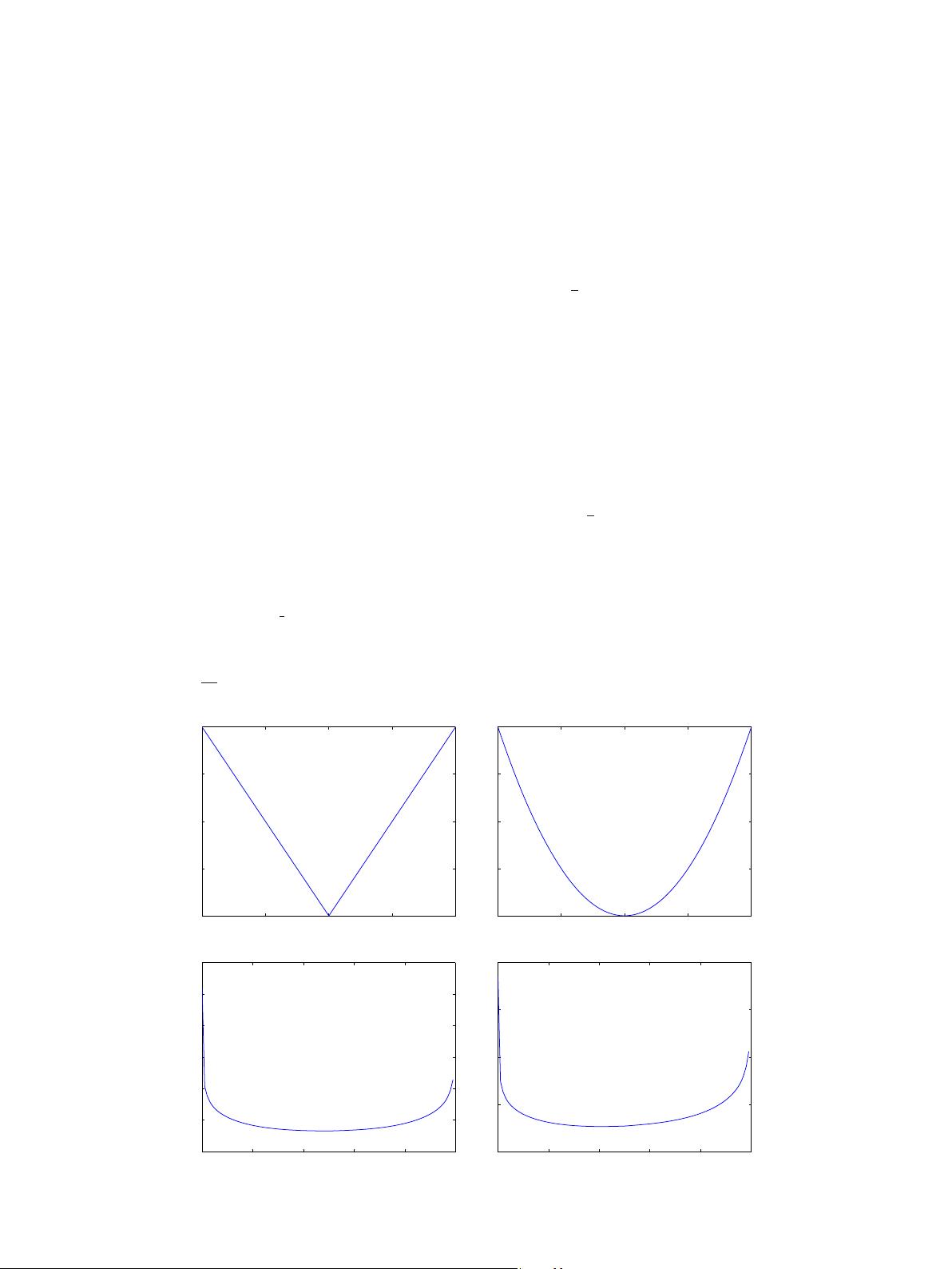
The Laplacian loss function, the Gaussian loss function and the
Beta loss function of parameters are shown in Fig. 2.
Give samples D
l
, we construct a nonlinear regression function
f ðxÞ¼
ω
T
ΦðxÞþb. The uniform model of kernel ridge regression
technique for the general noise model (N-KRR) can be formally
defined as
min g
P
N KRR
¼
1
2
ω
T
ωþ C ∑
l
i ¼ 1
cðe
i
Þ
()
P
N KRR
: s:t: y
i
ω
T
Φðx
i
Þb ¼ e
i
ði ¼ 1; …; lÞ; ð9Þ
cðe
i
ÞZ 0ði ¼ 1; 2; …; lÞ are general convex loss functions in the
sample point ðx
i
; y
i
ÞA D
l
. C 4 0 is a penalty parameter.
We construct a Lagrangian function from the primal objective
function and the corresponding constraints by introducing a dual
set of variables. Standard Lagrangian techniques are used to derive
the dual problem.
Theorem 1. The dual problem of the primal problem (9) of N-KRR is
max g
D
N KRR
¼
1
2
∑
l
i ¼ 1
∑
l
j ¼ 1
ðα
i
α
j
Kðx
i
; x
j
ÞÞ
(
þ ∑
l
i ¼ 1
ðα
i
y
i
ÞþC ∑
l
i ¼ 1
ðTðe
i
ðα
i
ÞÞ
)
ð10Þ
D
N KRR
: s:t: ∑
l
i ¼ 1
α
i
¼ 0;
where Tðe
i
ðα
i
ÞÞ ¼ cðe
i
ðα
i
ÞÞe
i
ðα
i
Þ∂ðcðe
i
ðα
i
ÞÞÞ=∂ðe
i
ðα
i
ÞÞ, e
i
is a func-
tion of variable
α
i
(i ¼ 1; …; l), C 4 0 is constant.
−2 −1 0 1 2
0
0.5
1
1.5
2
Laplacian Loss function
−2 −1 0 1 2
0
0.5
1
1.5
2
Gaussian Loss function
0 0.2 0.4 0.6 0.8 1
0
10
20
30
40
50
60
Beta Loss function,m=n=5.5
0 0.2 0.4 0.6 0.8 1
0
5
10
15
20
Beta Loss function,m=2.6084,n=3.0889
Fig. 2. Laplacian loss function, Gaussian loss function and Beta loss function of parameters.
S. Zhang et al. / Neurocomputing 149 (2015) 836–846838
剩余10页未读,继续阅读
497 浏览量
115 浏览量
318 浏览量
131 浏览量
340 浏览量
102 浏览量
358 浏览量
171 浏览量
点击了解资源详情

weixin_38587924
- 粉丝: 4
 我的内容管理
展开
我的内容管理
展开


最新资源
- Openaea:Unity下开源fanmad-aea游戏开发
- Eclipse中实用的Maven3插件指南
- 批量查询软件发布:轻松掌握搜索引擎下拉关键词
- 《C#技术内幕》源代码解析与学习指南
- Carmon广义切比雪夫滤波器综合与耦合矩阵分析
- C++在MFC框架下实时采集Kinect深度及彩色图像
- 代码研究员的Markdown阅读笔记解析
- 基于TCP/UDP的数据采集与端口监听系统
- 探索CDirDialog:高效的文件路径选择对话框
- PIC24单片机开发全攻略:原理与编程指南
- 实现文字焦点切换特效与滤镜滚动效果的JavaScript代码
- Flask API入门教程:快速设置与运行
- Matlab实现的说话人识别和确认系统
- 全面操作OpenFlight格式的API安装指南
- 基于C++的书店管理系统课程设计与源码解析
- Apache Tomcat 7.0.42版本压缩包发布
