深度学习:理解与应用——领域适应与迁移学习入门
需积分: 10 43 浏览量
更新于2024-07-16
收藏 700KB PDF 举报
在"An introduction to domain adaptation and transfer learning.pdf"这篇技术报告中,作者Wouter M. Kouw和Marco Loog探讨了在深度学习和机器学习背景下,当训练数据与潜在分布存在偏差时,如何处理数据分布变化的问题。通常,如果训练数据代表了底层数据分布,学习到的分类函数能在新样本上做出准确预测。然而,现实情况中,训练数据与测试数据之间的分布差异可能导致标准分类器在测试阶段表现不佳。
报告的核心内容围绕“域适应”和“迁移学习”这两个机器学习子领域展开。域适应关注的是在源域(训练数据的来源)和目标域(应用或测试数据的环境)之间,如何使分类器能够适应数据分布的变化,从而提高泛化能力。迁移学习则是在源域的知识或模型中寻找有价值的信息,以便在没有直接相关训练数据的目标任务中应用。
报告首先介绍了风险最小化的基本概念,这是理解转移学习和域适应理论框架的关键。风险最小化目标是通过优化模型参数来最小化预测错误的概率,这对于确保模型的稳定性和有效性至关重要。接下来,作者深入讨论了如何通过迁移学习扩大风险最小化的应用范围,例如,通过特征选择、权重调整或元学习等策略,将源域的模型或知识迁移到目标任务中,以减少对目标域大量标注数据的需求。
然后,报告会探讨不同类型的域适应方法,如自适应学习、半监督学习、无监督学习以及合成域方法,这些方法针对不同的场景和数据条件,提供了灵活的解决方案。此外,报告还可能涉及一些经典案例研究,展示在图像识别、自然语言处理等实际问题中,如何有效地进行域适应和迁移学习。
最后,作者总结了当前领域的挑战与前景,如开放世界假设、跨领域性能评估标准的制定,以及未来可能的研究方向,比如集成多源知识、动态适应和对抗性域适应等。这份报告为读者提供了一个全面的入门指南,帮助理解如何在面临数据分布不一致时,通过转移学习和域适应技术提升机器学习模型的泛化能力和实用性。

8 W.M. Kouw, M. Loog
Generalization Ultimately, we are not interested in the error of the trained
classifier on the given data set, but in the error on all possible future sa mples
e(h) = E
X ,Y
[h(x) 6= y]. The differe nc e between the true error and the empirical
error is known as the generalization error: e(h)− ˆe(h) [11,151]. Ideally, we would
like to know if the gener alization error will be small, i.e., that our classifier will
be approximately correct. However, because classifiers are functions of data sets,
and data sets are random, we can o nly de scribe how probable it is that our
classifier will be approximately correct. We can say that, with probability 1 − δ,
where δ > 0, the following inequality bolds (Theorem 2.2 from [151]):
e(h) − ˆe(h) ≤
r
1
2n
log |H | + log
2
δ
. (2)
where |H| denotes the cardinality of the finite hypothesis spac e, or the number
of classification functions that are being considered [193,119,151]. This result
is known as a Probably Approximately Corre c t (PAC) bound. In words, the
difference between the true error, e(h), and the empirical error, ˆe(h), of a classifier
is less than the square root of the logarithm of the size of the hypothesis space
|H|, plus the log of 2 over δ, normalized by twice the sample size n. In order to
achieve a similar result fo r the case of an infinite hypothesis spa c e (e.g. line ar
classifiers ), a measure of the c omplexity of the hypothesis space is r equired.
Generalization error bounds are interesting because they analyze what a clas-
sifier’s performance depends on. In this case, it suggest choo sing a smaller or
simpler hypothesis space when the sample size is low. Many variants of bounds
exist. Some use different measures of complexity, such as Rademacher complex-
ity [14] or Vapnik-Chervonenkis dimensions [20,197], while others use concepts
from Bayesian inference [147,131,15].
Bounds can incorporate assumptions on the pr oblem setting [12,151,54]. For
example, one can assume that the posterior distributions in each domain are
equal a nd obtain a bound for a classifier that exploits that assumption (c.f.
Equation 6). Assumptions restrict the problem setting, i.e., settings where that
assumption is invalid are disre garded. This often means that the bound is tighter
and a more accurate desc ription of the behaviour of the classifier can be found.
Such results have inspired new algor ithms in the past, such as Adaboost or the
Support Vector Machine [69,47].
Regularization Generalization error bounds tell us that the complexity, or
flexibility, of a c lassifier has to be traded off with the number of available train-
ing s amples [61,197,54]. In particular, a flexible model c an minimize the error
on a given data set completely, but will be too specific to generalize to new
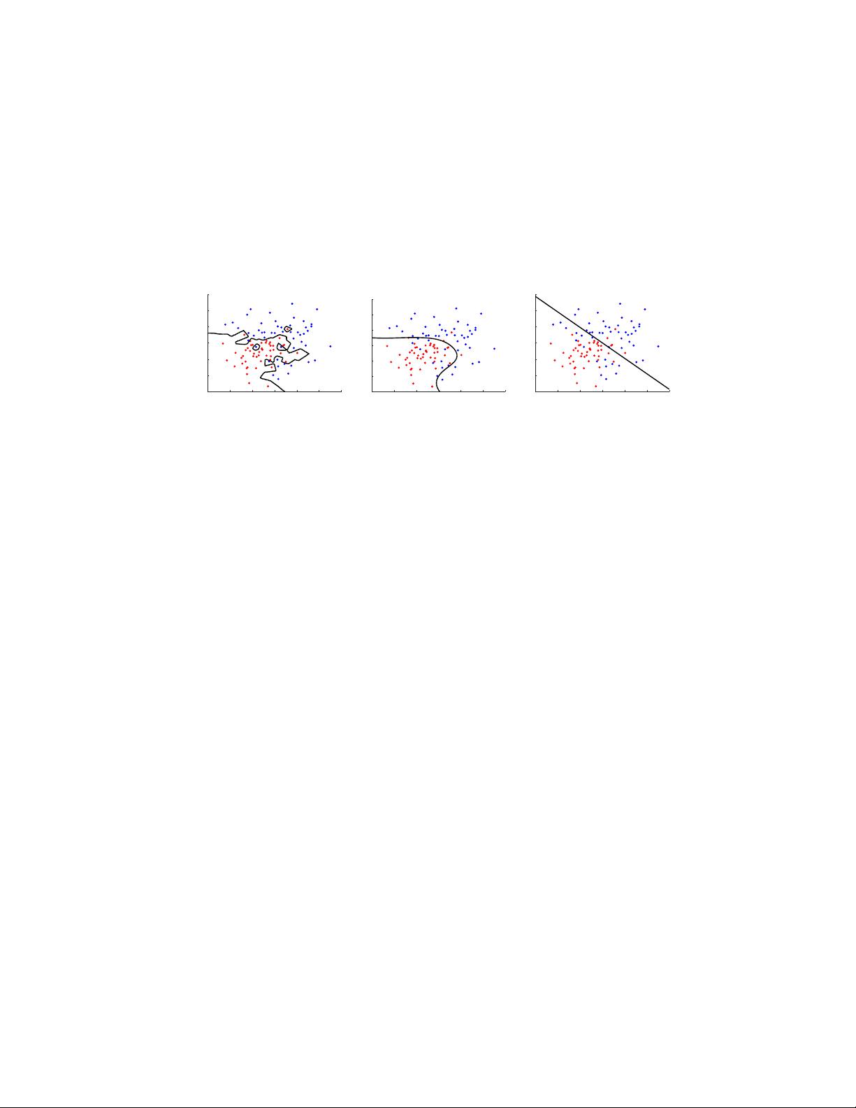
samples. This is known as overfitting. Figure 2 (left) illustrates an example of
2-dimensional classification problem with a classifier that ha s perfectly fitted to
the training set. As can be imagined, it will not perform as well for new s amples.
In order to combat overfitting, an additional term is introduced in the empiric al
剩余41页未读,继续阅读
点击了解资源详情
441 浏览量
点击了解资源详情
460 浏览量
588 浏览量
点击了解资源详情
点击了解资源详情
点击了解资源详情
点击了解资源详情

dywlegend1002
- 粉丝: 1
 我的内容管理
展开
我的内容管理
展开


最新资源
- 自动生成CAD模型文件的测试流程
- 掌握JavaScript中的while循环语句
- 宜科高分辨率编码器产品手册解析
- 探索3CDaemon:FTP与TFTP的高效传输解决方案
- 高效文件对比系统:快速定位文件差异
- JavaScript密码生成器的设计与实现
- 比特彗星1.45稳定版发布:低资源占用的BT下载工具
- OpenGL光源与材质实现教程
- Tablesorter 2.0:增强表格用户体验的分页与内容筛选插件
- 设计开发者的色值图谱指南
- UYA-Grupo_8研讨会:在DCU上的培训
- 新唐NUC100芯片下载程序源代码发布
- 厂家惠新版QQ空间访客提取器v1.5发布:轻松获取访客数据
- 《Windows核心编程(第五版)》配套源码解析
- RAIDReconstructor:阵列重组与数据恢复专家
- Amargos项目网站构建与开发指南
