
Interferences.
Methylene chloride
or
chloroform-soluble carboxylic acids
(acetylsalicylic acid, salicylic acid,
etc.) which inhibited 4-,UP response
were readily extracted from these
phases using
0.ln’
sodium hydroxide.
Span-type excipients, which gave
a
slight response
to
the 4-AAP reagent,
were eliminated by virtue of their insol-
ubility in
10%
aqueous sodium chloride;
while interfering Tween-type excipients
were precipitated
(3)
using the Tween
reagent. Propylene glycol, when formu-
lated at
a
level of
5.25%,
contributed ca.
2 to
370
to the observed absorbance.
This was minimized by
a
more favorable
distribution of the interference within
the aqueous phases used in the pro-
cedure.
Placebo analyses indicated that no
interference was obtained with such
common excipients
as
stearic acid,
stearyl alcohol, cetyl alcohol, petrola-
tum, methyl or propyl-p-hydroxy-
benzoates, sesame oil, or thimerosal.
Lipotropic agents (betaine or choline),
all the common vitamins, and neomycin
sulfate failed to interfere.
Scope
of
Reaction.
In addition to
the other types of steroids reported
to react with the 4-AAP reagent, the
following steroids reacted at elevated
temperature (boiling point of methanol)
and at increased concentration (2.0 mg.
per
10.0
ml. of reagent): 2a-hydroxy-
methyl
-
17p
-
hydroxy
-
17a
-
methyl-
5a-androst-%one (306 mp)
;
and 2a-
hydroxymethyl
-
17p
-
hydroxy
-
501-
androst-3-one (306 mp). Steroids with-
out
a
keto group failed to give any
response. The quantitative aspects of
the above responses to the 4-AAP
reagent were not investigated.
Correlations
of
Chromophore Wave-
length with Structure.
The additive
effect of various ring
A
and
B
sub-
stituents on the chromophore of the
parent saturated-3-keto steroid is
presented in Table
11.
LITERATURE CITED
(1)
Cohen,
H.,
Bates,
R.
W.,
J.
Am.
Pharm.
Assoc.,
Sci.
Ed.
40, 35 (1951).
(2) Hiittenrauch,
R.,
Z.
Physiol. Chem.
326,166 (1961).
(3) Pitter, P.,
Chem.
&
Ind.
42, 1832
(1962).
RECEIVED
for
review September 4, 1963.’
Accepted March 13,
1964.
Smoothing and Differentiation
of
Data
by
Simplified Least Squares Pro,cedures
ABRAHAM SAVITZKY and MARCEL
J.
E.
GOLAY
The Perkin-Elmer Corp., Norwalk, Conn.
b
In attempting to analyze, on
dig i ta
I
computers, data
f
rom basica
II
y
continuous physical experiments,
numerical methods of performing fa-
miliar operations must be developed.
The operations of differentiation and
filtering are especially important both
as an end in themselves, and as a pre-
lude to further treatment of the data.
Numerical counterparts
of
analog de-
vices that perform these operations,
such as RC filters, are often considered.
However, the method of least squares
may be used without additional com-
putational complexity and with con-
siderable improvement in the informo-
tion obtained. The least squares cal-
culations may be carried out in the
computer by convolution of the data
points with properly chosen sets
of
integers. These sets of integers and
their normalizing factors are described
and their use
is
illustrated in spectro-
scopic applications. The computer
programs required are relatively sim-
ple. Two examples are presented as
subroutines in the FORTRAN language.
HE
PRIMARY
OUTPUT
of any experi-
Tment in which quantitative
information is to be extracted is infor-
mation which measures the phenomenon
under observation. Superimposed upon
and indistinguishable from this informa-
tion are random errors which, regardless
of their source, are characteristically
described as noise. Of fundamental
importance
to
the esperimenter is the
removal of as much of this noise
as
possible without,
at
the same time,
unduly degrading the underlying in-
formation.
In much experimental work, the infor-
mation may be obtained in the form of
a
two-column table of numbers,
A
us.
B.
Such a table is typically the result
of
digitizing
a
spectrum
or
digitizing other
kinds of results obtained during the
course of an experiment.
If
plotted,
this table of numbers would give the
familiar graphs of
TOT
us.
wavelength,
pH
us.
volume of titrant, polarographic
current
us.
applied voltage,
SMR
or
ESR
spectrum,
or
chromatographic
elution curve, etc. This paper is con-
cerned with computational methods for
the removal of the random noise from
such information, and with the simple
evaluation of the first few derivatives
of the information with respect to the
graph abscissa.
The bases for the methods
to
be dis-
cussed have been reported previously,
mostly in the mathematical literature
(4,
6,
8,
9).
The objective here is to
present specific methods for handling
current problems in the processing of
such tables of analytical data. The
methods apply as well to the desk
calculator,
or
to simple paper and pencil
operations for small amounts of data, as
they do to the digital computer for
large amounts of data, since their major
utility is to simplify and speed up the
processing of data.
There are two important restrictions
on the way in which the points in the
table may be obtained. First, the points
must be at
a
fixed, uniform interval in
the chosen abscissa.
If
the independent
variable is time, as in chromatography
or
NMR
spectra with linear time sweep,
each data point must be obtained at the
same time interval from each preceding
point.
If
it
is
a
spectrum, the intervals
may be every drum division
or
every
0.1
wavenumber, etc. Second, the
curves formed by graphing the points
must be continuous and more
or
less
smooth-as in the various examples
listed above.
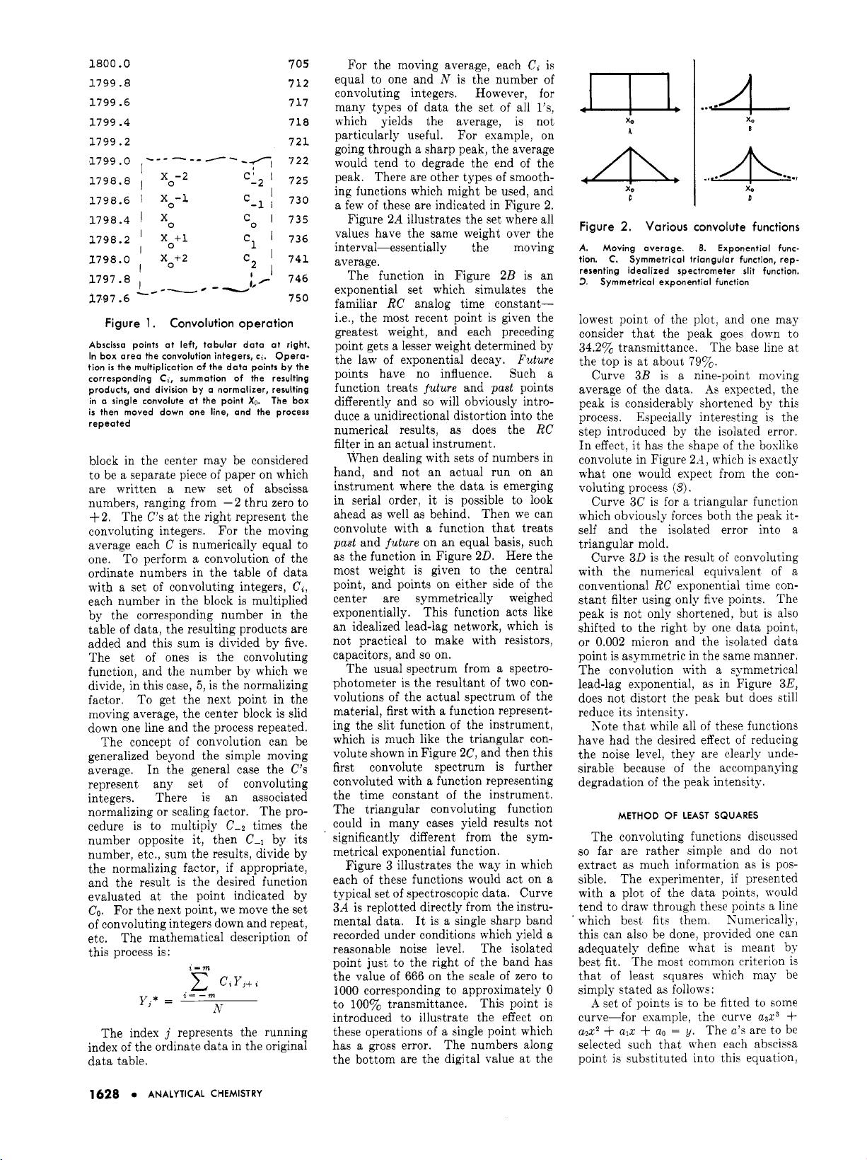
ALTERNATIVE METHODS
One of the simplest ways to smooth
fluctuating data is by a moving average.
In this procedure one takes
a
fised
number of points, adds their ordinates
together, and divides by the number
of
points to obtain the average ordinate at
the center abscissa of the group. Sest,
the point at one end of the group is
dropped, the next point at the other end
added, and the process is repeated.
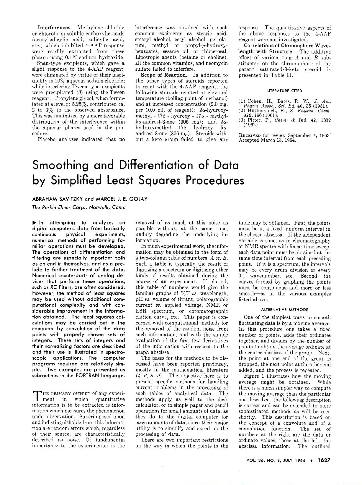
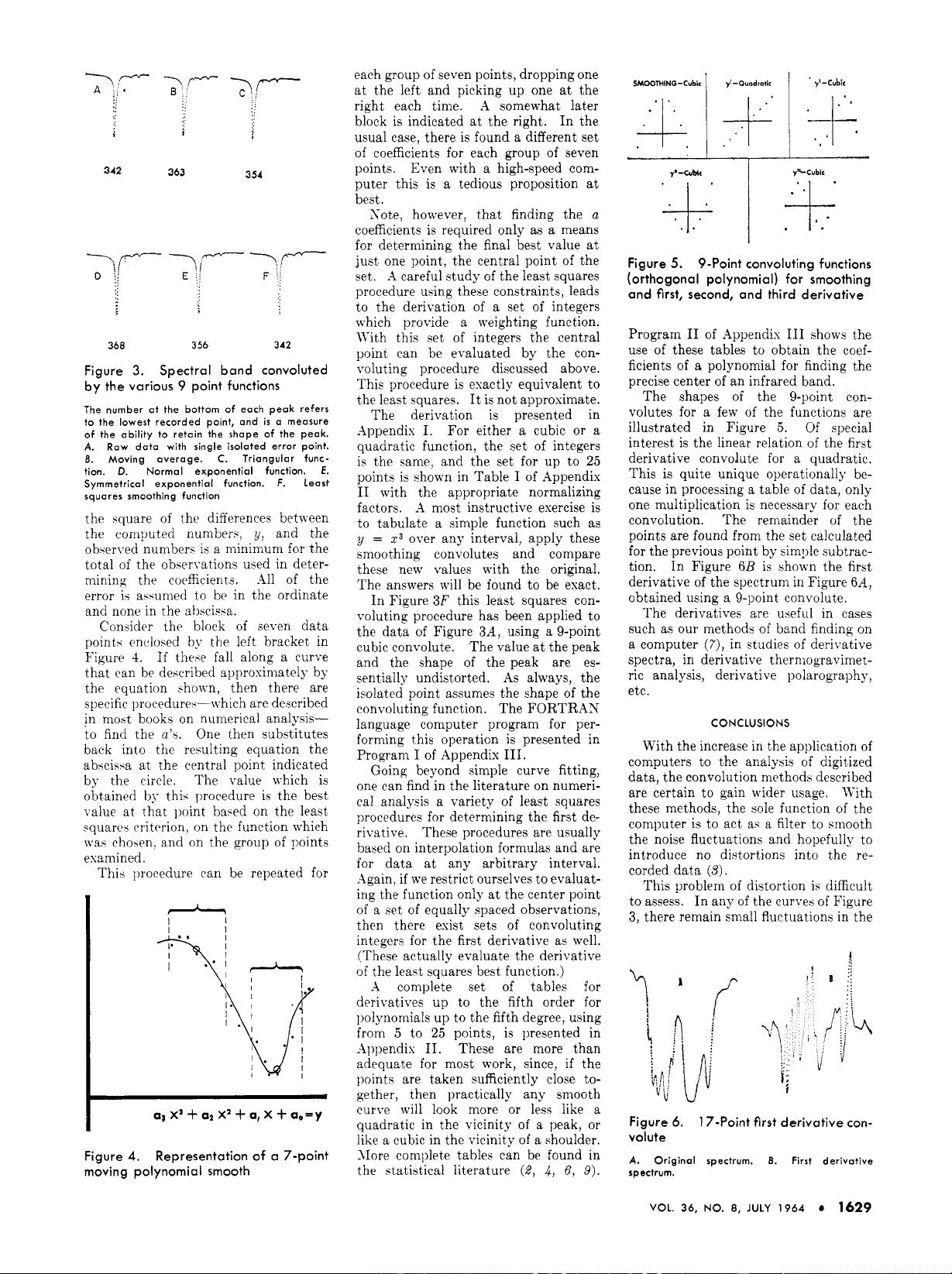
Figure
1
illustrates how the moving
average might be obtained. While
there is a much simpler way to compute
the moving average than the particular
one described, the following description
is correct and can be extended to more
sophisticated methods as will be seen
shortly. This description is based on
the concept of a convolute and of a
convolution function. The set of
numbers at the right are the data or
ordinate values, those at the left, the
abscissa information. The outlined
VOL.
36,
NO.
8,
JULY
1964
1627
剩余12页未读,继续阅读

kerwinliu
- 粉丝: 32
- 资源: 5
 我的内容管理
收起
我的内容管理
收起
- 我的资源
快来上传第一个资源
 我的收益 登录查看自己的收益
 我的积分
登录查看自己的积分
我的积分
登录查看自己的积分
 我的C币
登录后查看C币余额
我的C币
登录后查看C币余额
 我的收藏
我的收藏  我的下载
我的下载  下载帮助
下载帮助

会员权益专享


最新资源
- RTL8188FU-Linux-v5.7.4.2-36687.20200602.tar(20765).gz
- c++校园超市商品信息管理系统课程设计说明书(含源代码) (2).pdf
- 建筑供配电系统相关课件.pptx
- 企业管理规章制度及管理模式.doc
- vb打开摄像头.doc
- 云计算-可信计算中认证协议改进方案.pdf
- [详细完整版]单片机编程4.ppt
- c语言常用算法.pdf
- c++经典程序代码大全.pdf
- 单片机数字时钟资料.doc
- 11项目管理前沿1.0.pptx
- 基于ssm的“魅力”繁峙宣传网站的设计与实现论文.doc
- 智慧交通综合解决方案.pptx
- 建筑防潮设计-PowerPointPresentati.pptx
- SPC统计过程控制程序.pptx
- SPC统计方法基础知识.pptx
资源上传下载、课程学习等过程中有任何疑问或建议,欢迎提出宝贵意见哦~我们会及时处理!
点击此处反馈


评论0